yt: Astrophysically-Aware Analysis and Viz Matthew Turk (Columbia) - PowerPoint PPT Presentation

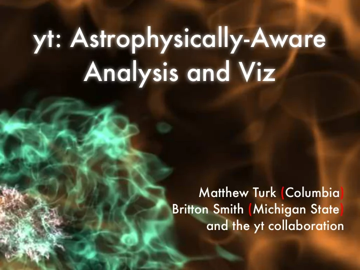
yt: Astrophysically-Aware Analysis and Viz Matthew Turk (Columbia) Britton Smith (Michigan State) and the yt collaboration

First, some motivation.

the stars

how to make a star

76% 24%

hydrodynamics

(example)

There is only one sky. (but there are many simulation codes)

Different methods, data structures, assumptions, IO methods, units, variable names, ...

Analysis.

astro-ph/1011.3514 yt-project.org

install script: Full dependency stack Source code Development environment GUI Sample data

yt has been designed to address physical, not computational, entities.

The Universe is full of gas, dark matter and stars. yt makes it easy to access that material.

Transparent IO, masking of overlapping data, load-on-demand, geometric and non- geometric selection, field generation, and common interfaces to different datatypes.

Enzo, Orion, CASTRO, FLASH Chombo, Tiger, Athena , ART, RAMSES yt is designed to be the lingua franca of astrophysical codes.

Objects (conceptual, uniformly accessible NumPy stores)

Objects Orthogonal Rays 1D Non-orthogonal Rays Slices Oblique Slices 2D Projections Spheres Rectangular Prisms Disks/Cylinders Inclined Boxes 3D Clumps Extracted Regions Boolean combinations

Objects All respect unified interface: from yt.mods import * pf = load(“DataDump0155.dir/DataDump0155”) ray = pf.h.ray([0.1, 0.2, 0.5], [0.4, 0.9, 0.1]) print ray[“Density”]

Objects All respect unified interface: from yt.mods import * pf = load(“DataDump0155.dir/DataDump0155”) sl = pf.h.slice(0, 0.5) print sl[“Density”]

Objects All respect unified interface: from yt.mods import * pf = load(“DataDump0155.dir/DataDump0155”) sp = pf.h.sphere(100.0/pf[‘au’], ‘max’) print sp[“Density”]

from yt.mods import * pf = load(“DataDump0155.dir/DataDump0155”) v, c = pf.h.find_max(“Density”)

Adding new fields should be easy.

from yt.mods import * @derived_field(“Pressure”) def Pressure(field, data): return (data.pf["Gamma"] - 1.0) * \ data["Density"]*data["ThermalEnergy"]

Scripts should be simple and clear.

from yt.mods import * pf = load(“DataDump0155.dir/DataDump0155”) pc = PlotCollection(pf) pc.add_phase_sphere(1000.0, ‘au’, [“Density”, “Temperature”, “H2I_Fraction”]) pc.save()

from yt.mods import * pf = load(“DataDump0155.dir/DataDump0155”) pc = PlotCollection(pf) pc.add_phase_sphere(1000.0, ‘au’, [“Density”, “Temperature”, “CellMassMsun”], weight = None) pc.save()

from yt.mods import * pf = load(“DataDump0155.dir/DataDump0155”) pc = PlotCollection(pf) pc.add_slice(“Density”, 0) pc.set_width(0.5, ‘unitary’) pc.save()

from yt.mods import * pf = load(“DataDump0155.dir/DataDump0155”) pc = PlotCollection(pf) pc.add_slice(“Density”, 0) pc.set_width(1.0, ‘pc’) pc.save()

from yt.mods import * pf = load(“DataDump0155.dir/DataDump0155”) pc = PlotCollection(pf) pc.add_slice(“Density”, 0) pc.set_width(1000.0, ‘au’) pc.save()

Some Highlights!

(px, py, pdx, pdy, z) Projections

(px, py, pdx, pdy, z) Image Buffer

(px, py, pdx, pdy, z) Image Buffer

Project once, pixelize many

Slices

Oblique Slices

Isocontour Extraction

Parallelism

Parallelism Embarassingly Parallel Spatial Decomposition Decomposed by load or Helper functions to IO characteristics decompose the domain

Parallelism Embarassingly Parallel Spatial Decomposition Quantities Profiles Slices Halo Finding Projections Volume Rendering

Multi-level parallelism: dynamic workgroups, communicators, subgroups and task queues

Volume Rendering

Designed around integrating through a volume: visualization is a side effect. dI ν ds = j ν − α ν I ν

Credit: Sam Skillman, 3rd Place at SciDAV Viz Night

from yt.mods import * pf = load(“DataDump0155.dir/DataDump0155”) v, c = pf.h.find_max("Density") L = [1.0, 1.0, 1.0] W = 1000.0/pf['au'] tf = vr.ColorTransferFunction((-14.0, -4)) tf.add_layers(8) cam = pf.h.camera(c, L, W, 1024, tf) cam.snapshot()

from yt.mods import * pf = load(“DataDump0155.dir/DataDump0155”) v, c = pf.h.find_max("Density") sp = pf.h.sphere(c, 1000.0/pf['au']) L = sp.quantities["AngularMomentumVector"]() W = 1000.0/pf['au'] tf = vr.ColorTransferFunction((-14.0, -4)) tf.add_layers(8) cam = pf.h.camera(c, L, W, 1024, tf) cam.snapshot()

cam.zoom(100.0) cam.snapshot()

from yt.mods import * pf = load(“DD1701/DD1701”) v, c = pf.h.find_max("Density") L = [1.0, 1.0, 1.0] W = 100.0/pf['mpc'] tf = vr.PlanckTransferFunction() cam = pf.h.camera(c, L, W, 1024, tf) cam.snapshot()

Off-axis Projection

Canned Analysis Tasks

Absorption Spectrum Coordinate Transformations Halo Finding Mass Functions Merger Trees Halo Profiling Level Sets Light Cones Light Rays Time Series Star Analysis Two-Point Analysis

Level Sets

Synthetic Spectra

Two-Point Functions

Three Halo Finders: Standard HOP Friends of Friends Parallel HOP Rockstar (beta)

co-scheduled & in situ viz

Process Simulation yt Thin NumPy wrappers and stop-n-go

On Disc → In-situ

Inter-comm Simulation yt Fire and forget, no embedded interpreter

Developing as a Team

Code review: eyes on (nearly) every changeset

Forky development: very low barrier to entry; everything comes in the box.

Testing: answer as well as integration tests get run every 30 minutes.

80,000 lines of code Python, Cython, C 20 contributors (60+ users) Contributors from 10+ institutions 8AM 6PM

Challenges

Low bus factor.

Chores nobody wants to do.

The import problem!

What’s next?

initialization

better astrophysical object selection

solvers

non-astrophysical data