You have studied bill width in a population of finches for many - PDF document

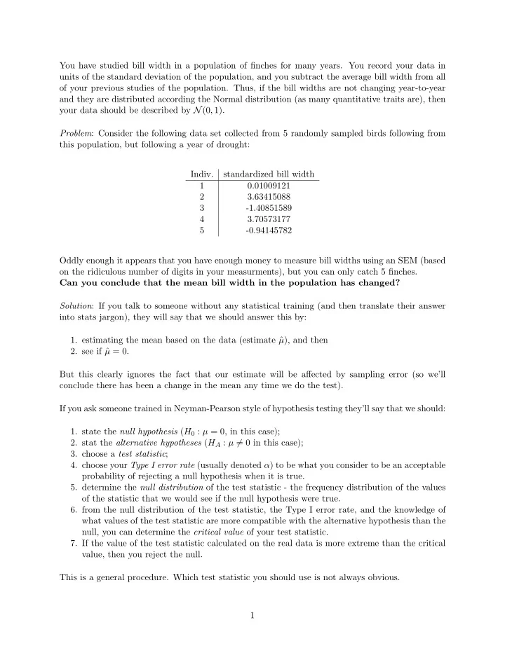
You have studied bill width in a population of finches for many years. You record your data in units of the standard deviation of the population, and you subtract the average bill width from all of your previous studies of the population. Thus, if the bill widths are not changing year-to-year and they are distributed according the Normal distribution (as many quantitative traits are), then your data should be described by N (0 , 1). Problem : Consider the following data set collected from 5 randomly sampled birds following from this population, but following a year of drought: Indiv. standardized bill width 1 0.01009121 2 3.63415088 3 -1.40851589 4 3.70573177 5 -0.94145782 Oddly enough it appears that you have enough money to measure bill widths using an SEM (based on the ridiculous number of digits in your measurments), but you can only catch 5 finches. Can you conclude that the mean bill width in the population has changed? Solution : If you talk to someone without any statistical training (and then translate their answer into stats jargon), they will say that we should answer this by: 1. estimating the mean based on the data (estimate ˆ µ ), and then 2. see if ˆ µ = 0. But this clearly ignores the fact that our estimate will be affected by sampling error (so we’ll conclude there has been a change in the mean any time we do the test). If you ask someone trained in Neyman-Pearson style of hypothesis testing they’ll say that we should: 1. state the null hypothesis ( H 0 : µ = 0, in this case); 2. stat the alternative hypotheses ( H A : µ � = 0 in this case); 3. choose a test statistic ; 4. choose your Type I error rate (usually denoted α ) to be what you consider to be an acceptable probability of rejecting a null hypothesis when it is true. 5. determine the null distribution of the test statistic - the frequency distribution of the values of the statistic that we would see if the null hypothesis were true. 6. from the null distribution of the test statistic, the Type I error rate, and the knowledge of what values of the test statistic are more compatible with the alternative hypothesis than the null, you can determine the critical value of your test statistic. 7. If the value of the test statistic calculated on the real data is more extreme than the critical value, then you reject the null. This is a general procedure. Which test statistic you should use is not always obvious. 1

The Neyman-Pearson lemma states that we should use the likelihood ratio test-statistic if we are testing two distinct points (e.g. if H 0 : µ = 0 and H A : µ = 1 for example). The lemma actually states that the likelihood ratio test-statistic is the most powerful (e.g. gives us the most power to reject the null when it is false) that is “honest” in the sense of guaranteeing it reported Type I error rate. In our case, we do not have a distinct hypothesis (“point hypothesis”) as an alternative. But we can still use the likelihood ratio as our test statistic, but we have to have a pair of points to use when calculating the test statistic. We can use the MLE when calculating the likelihood that is in the denominator in the ratio, and we can use the null hypothesis’ value of µ when calculating the numerator. We also take the log of the ratio and multiply it by -2 (so that the properties that we proved in problem #3 of homework #2 hold): − 2 ln Λ = 2 ln[ L (ˆ µ )] − 2 ln[ L ( µ 0 )] . As you may recall from the second homework: L ( µ ) = Pr( X | µ ) n � = Pr( x i | µ ) i =1 n 2 πσ 2 e − ( xi − µ )2 1 � = √ 2 σ 2 i =1 If we assume that σ = 1 then we also showed that: � n � x 2 xµ − nµ 2 � � 1 � i √ ln[ L ( µ )] = n ln − + n ¯ 2 2 2 π i =1 � n i x µ ˆ = x = ¯ n For the data set shown above ˆ µ = ¯ x = 1, and our null dictates that µ 0 = 0. We can also calculate � � that: 0 . 5 ∗ � 5 i =1 x 2 1 i = 14 . 90493 and 5 ln = 4 . 59469 for our data set. This lets us conveniently √ 2 π express the log-likelihood as: � 5 � − 5 µ 2 � ln[ L ( µ )] = 19 . 49962 + x i µ 2 i =1 19 . 49962 + 5 µ − 5 µ 2 ln[ L ( µ )] = 2 19 . 49962 + µ − 2 . 5 µ 2 = � n i x µ ˆ = x = ¯ n ln[ L ( µ 0 )] = − 19 . 4996 ln[ L (ˆ µ )] = − 16 . 9996 − 2 ln Λ = 5 2

You will recall (from lecture and the homework) that know the null distribution of the LR test statistic in cases like this one (in which the MLE is not at a boundary, we are test a general model against a more specific “nested” form of the model, and the likelihood curve looks like a normal). The null distribution is simply χ 2 k where the degrees of freedom, k , is simply to the number of parameters that are free to vary in the more complex (less constrained) model ( H A ) but are fixed in the more simple model ( H 0 ). The critical value for χ 2 1 = 3 . 84. Our observed test statistic is greater than this, so we can reject the null. It may be helpful to plot the ln[ L ( µ )] for different values of µ . In this case the plot is simply a parabola with the maximum point at µ = 1: � 18 � 20 � 22 � 24 � 26 � 28 � 1 1 2 3 4 the horizontal line is at -18.9196, which is 1.92 below the maximum likelihood score. 1.92 is chosen because twice this value corresponds to 3.84 (our critical value). If we were to test a null hypothesis that µ takes a particular value, and the log-likelihood is below this threshold then we could reject the null 1 . This means that we could construct a 95% confidence interval based on where the log-likelihood intersects with the threshold score. In this case, the confidence interval would be 0 . 123644 ≤ µ ≤ 1 . 87636, which does not include our null point ( µ = 0). Let us pause a note that we just did a hypothesis test, but we could also view this as an exercise in model selection. We contrasted a zero-parameter model N (0 , 1) to a one-parameter model, N ( µ, 1), and asked whether we could reject the simpler model.- This is the likelihood-ratio test approach to model testing. Essentially the attitude is: only use a more complex model if the data warrants it, and we can assess this by performing a hypothesis test. If we reject the simpler model, then we feel justified in using the more complex model. OK, so it appears that we have evidence that the mean bill width has changed 2 . But if we have evidence that the distribution of bill widths has changed, can we really trust the applicability of the standard deviation from previous studies? 1 We are supposed to construct our null befor the test - this is just a thought experiment. 2 The use of the LR test statistic gives us confidence that we have used the most powerful test, but the fact that the LR is monotonic function of the distance between ¯ x and the hypothesized mean ( µ ) guarantees that we could have conducted an equally powerful test using ¯ x as our test statistic. So the typical Z-test that may have occurred to you is just as good as the LR test in this case. 3

It would be safer to admit that we don’t know the correct value of σ . We can do this, but we will have a likelihood function with multiple parameters: n 2 πσ 2 e − ( xi − µ )2 1 � L ( µ, σ ) = √ 2 σ 2 i =1 � n � x 2 σ 2 − nµ 2 � 1 � + n ¯ xµ � i √ − ln[ L ( µ, σ )] = n ln 2 σ 2 2 σ 2 σ 2 π i =1 �� n � � √ x 2 xµ − nµ 2 1 � � � i = − n ln σ 2 π − + n ¯ 2 σ 2 2 2 i =1 This likelihood function is defined over a 2-D space of parameter values. Specifically, −∞ < µ < ∞ and 0 ≤ σ < ∞ . We are interested in finding the maximum point. It could occur at a boundary of parameters (although in this case the only boundary is σ = 0 and clearly the data are not consistent with no variance in bill width, so that should not be a maximum likelihood point). For an “internal” (non-boundary) point when we have a continuous and differentiable log-likelihood we are looking for a point at which the slope of the log-likelihood with respect to each of the parameters is zero (and the second derivatives are negative). ∂ ln[ L ( µ, σ )] n ¯ σ − nµ x = ∂µ σ n ¯ σ − n ˆ x µ = 0 σ ˆ µ = ¯ x In general, the first derivative with respect to one parameter will be a function of the other param- eters. In this special case, the σ in the first derivative wrt µ cancel out. This makes some sense: µ is the “center” of the distribution. While changing the variance of the model will affect how well it fits the data, it won’t make us change where we think the center of the distribution is. So the MLE of µ is simply ¯ x regardless of the value of σ . When we want to estimate ˆ σ we see that this is not the case: √ � n i =1 ( x i − µ ) 3 ∂ ln[ L ( µ, σ )] − n 2 π = √ 2 π + σ 2 ∂σ σ � n i =1 ( x i − µ ) 2 − n = σ + σ 3 � � n i =1 ( x i − µ ) 2 � 1 − n + = σ 3 σ � � � n i =1 ( x i − µ ) 2 1 − n + = 0 σ 2 σ ˆ ˆ σ becomes zero 3 or: The derivative equals zero if 1 / ˆ � n i =1 ( x i − µ ) 2 n = σ 2 ˆ 3 Because σ < ∞ this point is never reached. But it does make sense that as you increase the variance to huge values, the likelihood stops changing much. 4