Workshop 9.2a: Nested designs Murray Logan November 23, 2016 Table - PDF document

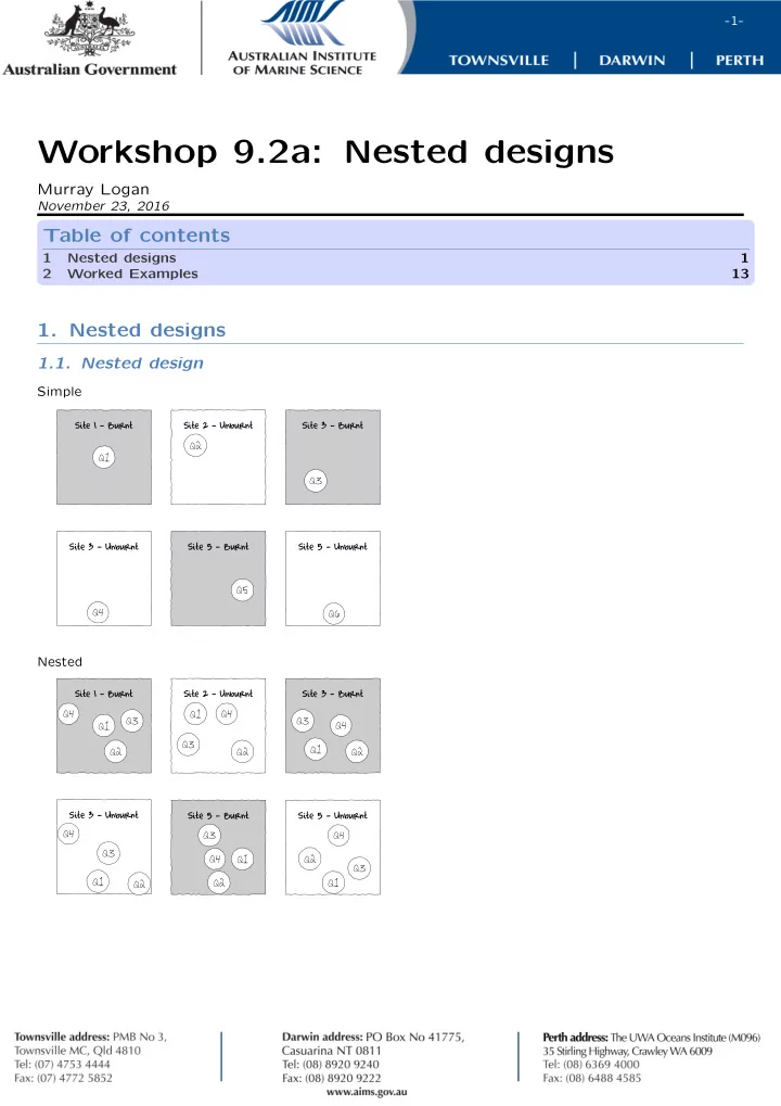
. . . . . . . . . . . . . . . . . . . . . . . . . . . . . . . . . . . . . . . . . . . . . . . . . . . . . . . . . . . . . . . . . -1- Workshop 9.2a: Nested designs Murray Logan November 23, 2016 Table of contents 1 Nested designs 1 2 Worked Examples 13 1. Nested designs 1.1. Nested design Simple Site 1 - Burnt Site 2 - Unburnt Site 3 - Burnt Q2 Q1 Q3 Site 3 - Unburnt Site 5 - Burnt Site 5 - Unburnt Q5 Q4 Q6 Nested Site 1 - Burnt Site 2 - Unburnt Site 3 - Burnt Q4 Q1 Q4 Q3 Q3 Q1 Q4 Q3 Q1 Q2 Q2 Q2 Site 3 - Unburnt Site 5 - Burnt Site 5 - Unburnt Q4 Q3 Q4 Q3 Q4 Q1 Q2 Q3 Q1 Q2 Q1 Q2

-2- 1.2. Nested design > data.nest <- read.csv('../data/data.nest.csv') > head(data.nest) y Region Sites Quads 1 32.25789 A S1 1 2 32.40160 A S1 2 3 37.20174 A S1 3 4 36.58866 A S1 4 5 35.45206 A S1 5 6 37.07744 A S1 6 1.3. Nested design > library(ggplot2) > data.nest$Sites <- factor(data.nest$Sites, levels=paste0('S',1:nSites)) > ggplot(data.nest, aes(y=y, x=1,color=Region)) + geom_boxplot() + + facet_grid(.~Sites) + + scale_x_continuous('', breaks=NULL)+theme_classic() S1 S2 S3 S4 S5 S6 S7 S8 S9 S10 S11 S12 S13 S14 S15 ● ● 100 80 Region A y ● B 60 C ● ● 40 ● ● 20 1.4. Nested design > #Effects of treatment > library(plyr) > boxplot(y~Region, ddply(data.nest, ~Region+Sites, + numcolwise(mean, na.rm=T)))

-3- 100 90 80 70 60 50 40 30 A B C 1.5. Nested design > #Site effects > boxplot(y~Sites, ddply(data.nest, ~Region+Sites+Quads, + numcolwise(mean, na.rm=T))) ● 100 ● 80 ● 60 ● 40 ● 20 S1 S3 S5 S7 S9 S11 S13 S15

. . . . . . . . . . . . . . . . . . . . . . . . . . . . . . . . . . . . . . . . . . -4- 1.6. Nested design Site 1 - Burnt Site 2 - Unburnt Site 3 - Burnt Q4 Q4 Q1 Q3 Q3 Q4 Q1 Q3 Q1 Q2 Q2 Q2 Site 3 - Unburnt Site 5 - Burnt Site 5 - Unburnt Q4 Q3 Q4 Q3 Q4 Q1 Q2 Q3 Q1 Q2 Q1 Q2 y = µ + α + β ( α ) + ϵ e.g. abundance = base + burnt + quadrat ( burnt ) 1.7. Nested design y = µ + α + β ( α ) + ϵ y ijk = µ + α i Region i + β j ( i ) Sites j ( i ) + ϵ ijk µ - base (mean of first Region) α - main fixed effect β - sub-replicates (Sites: random effect) > with(data.nest, table(Region,Sites)) Sites Region S1 S2 S3 S4 S5 S6 S7 S8 S9 S10 S11 S12 S13 S14 S15 A 10 10 10 10 10 0 0 0 0 0 0 0 0 0 0 B 0 0 0 0 0 10 10 10 10 10 0 0 0 0 0 C 0 0 0 0 0 0 0 0 0 0 10 10 10 10 10 > head(data.nest, 20) y Region Sites Quads 1 32.25789 A S1 1 2 32.40160 A S1 2 3 37.20174 A S1 3 4 36.58866 A S1 4 5 35.45206 A S1 5 6 37.07744 A S1 6 7 36.39324 A S1 7 8 32.85538 A S1 8 9 22.53580 A S1 9 10 35.58168 A S1 10 11 41.92308 A S2 11 12 41.42474 A S2 12

-5- 13 34.84996 A S2 13 14 39.81297 A S2 14 15 44.29343 A S2 15 16 48.99712 A S2 16 17 41.68978 A S2 17 18 44.14208 A S2 18 19 41.93469 A S2 19 20 35.31842 A S2 20 1.8. Nested design y = µ + α + β ( α ) + ϵ y ijk = µ + α i Region i + β j ( i ) Sites j ( i ) + ϵ ijk > library(nlme) > data.nest.lme <- lme(y~Region, random=~1|Sites, data.nest) > plot(data.nest.lme) 3 ● ● ● ● ● 2 ● ● ● ● ● ● ● Standardized residuals ● ● ● ● ● ● ● ● 1 ● ● ● ● ● ● ● ● ● ● ● ● ● ● ● ● ● ● ● ● ● ● ● ● ● ● ● ● ● ● ● ● ● ● ● ● ● ● ● ● ● ● ● ● ● ● ● ● ● ● ● ● ● ● ● 0 ● ● ● ● ● ● ● ● ● ● ● ● ● ● ● ● ● ● ● ● ● ● ● ● ● ● ● ● ● ● ● ● ● ● ● ● ● ● ● ● ● ● ● ● ● ● ● ● ● ● ● ● −1 ● ● ● ● ● ● ● ● ● ● ● ● ● ● ● ● ● ● ● ● ● −2 ● ● 40 60 80 100 Fitted values 1.9. Nested design > plot(data.nest$Region, residuals(data.nest.lme, + type='normalized'))

-6- ● ● 2 1 0 −1 −2 ● A B C 1.10. Nested design > summary(data.nest.lme) Linear mixed-effects model fit by REML Data: data.nest AIC BIC logLik 927.7266 942.6788 -458.8633 Random effects: Formula: ~1 | Sites (Intercept) Residual StdDev: 13.6582 4.372252 Fixed effects: y ~ Region Value Std.Error DF t-value p-value (Intercept) 42.27936 6.139350 135 6.886618 0.0000 RegionB 29.84692 8.682352 12 3.437654 0.0049 RegionC 37.02026 8.682352 12 4.263851 0.0011 Correlation: (Intr) ReginB RegionB -0.707 RegionC -0.707 0.500 Standardized Within-Group Residuals: Min Q1 Med Q3 Max -2.603787242 -0.572951701 0.004953998 0.620914933 2.765601716 Number of Observations: 150 Number of Groups: 15

-7- 1.11. Nested design > VarCorr(data.nest.lme) Sites = pdLogChol(1) Variance StdDev (Intercept) 186.54644 13.658200 Residual 19.11659 4.372252 > anova(data.nest.lme) numDF denDF F-value p-value (Intercept) 1 135 331.8308 <.0001 Region 2 12 10.2268 0.0026 1.12. Nested design > library(multcomp) > summary(glht(data.nest.lme, linfct=mcp(Region="Tukey"))) Simultaneous Tests for General Linear Hypotheses Multiple Comparisons of Means: Tukey Contrasts Fit: lme.formula(fixed = y ~ Region, data = data.nest, random = ~1 | Sites) Linear Hypotheses: Estimate Std. Error z value Pr(>|z|) B - A == 0 29.847 8.682 3.438 0.00172 ** C - A == 0 37.020 8.682 4.264 < 0.001 *** C - B == 0 7.173 8.682 0.826 0.68674 --- Signif. codes: 0 '***' 0.001 '**' 0.01 '*' 0.05 '.' 0.1 ' ' 1 (Adjusted p values reported -- single-step method) 1.13. Nested design > library(effects) > plot(allEffects(data.nest.lme))

-8- Region effect plot 90 80 ● ● 70 y 60 50 ● 40 30 A B C Region 1.14. Linear mixed effects model 1.14.1. Summary figure Step 1. gather model coefficients and model matrix > coefs <- fixef(data.nest.lme) > coefs (Intercept) RegionB RegionC 42.27936 29.84692 37.02026 > xs <- levels(data.nest$Region) > Xmat <- model.matrix(~Region, data.frame(Region=xs)) > head(Xmat) (Intercept) RegionB RegionC 1 1 0 0 2 1 1 0 3 1 0 1 1.15. Linear mixed effects model 1.15.1. Summary figure Step 3. calculate predicted y and CI > ys <- t(coefs %*% t(Xmat)) > head(ys)

-9- [,1] 1 42.27936 2 72.12628 3 79.29961 > SE <- sqrt(diag(Xmat %*% vcov(data.nest.lme) %*% t(Xmat))) > CI <- 2*SE > #OR > CI <- qt(0.975,length(data.nest$y)-2)*SE > data.nest.pred <- data.frame(Region=xs, fit=ys, se=SE, + lower=ys-CI, upper=ys+CI) > head(data.nest.pred) Region fit se lower upper 1 A 42.27936 6.13935 30.14725 54.41147 2 B 72.12628 6.13935 59.99417 84.25839 3 C 79.29961 6.13935 67.16751 91.43172 1.16. Linear mixed effects model 1.16.1. Summary figure Step 4. plot it > with(data.nest.pred,plot.default(Region, fit,type='n',axes=F, ann=F,ylim=range(c(data.nest.pred$lower, data.nest.pred$upper)))) > points(y~Region, data=data.nest, pch=16, col='grey') > points(fit~Region, data=data.nest.pred, pch=16) > with(data.nest.pred, arrows(as.numeric(Region),lower,as.numeric(Region),upper, length=0.1, angle=90, code=3)) > axis(1, at=1:3, labels=levels(data.nest$Region)) > mtext('Region',1,line=3) > axis(2,las=1) > mtext('Y',2,line=3) > box(bty='l') ● ● ● 90 ● ● ● ● ● ● ● ● ● ● ● ● ● ● ● ● ● ● ● 80 ● ● ● ● ● ● ● ● ● ● ● ● ● ● ● ● ● ● ● ● ● ● ● ● ● ● ● ● ● ● ● ● 70 ● ● ● ● ● ● ● ● ● ● ● ● ● ● ● ● ● ● ● ● ● ● Y ● ● ● ● 60 ● ● ● ● ● ● ● ● ● ● ● ● ● ● 50 ● ● ● ● ● ● ● ● ● ● ● ● ● ● ● ● ● ● ● 40 ● ● ● ● ● ● ● ● ● ● ● ● ● ● ● ● ● ● 30 ● ● ● ● ● A B C Region 1.17. Linear mixed effects model