Why is theory important? Heuristic Optimization We want to - - PowerPoint PPT Presentation

Heuristic Optimization

Lecture 5

Algorithm Engineering Group Hasso Plattner Institute, University of Potsdam

12 May 2015

Heuristic Optimization

Why is theory important?

We want to understand how an algorithm behaves over certain inputs. Idea: run the algorithm over a large set of instances and observe its behavior. Problem: sometimes evidence can be deceiving! Even when we think a process is well-behaved, it may not behave as we expect for all inputs.

12 May 2015 1 / 19 Heuristic Optimization

Why is theory important?

At least half of the natural numbers less than any given number have an

• dd number of prime factors.

— George P´

• lya (1919)

factor parity m < n = 20

• dd

even 19 16 = 24 18 = 2 · 32 15 = 3 · 5 17 14 = 2 · 7 13 10 = 2 · 5 12 = 22 · 3 9 = 32 11 6 = 2 · 3 8 = 23 4 = 22 7 5 3 2 Resolved (false) by C. Brian Haselgrove (1958). Smallest n for which the conjecture fails: n = 906 150 257 found by Minura Tanaka (1980).

12 May 2015 2 / 19 Heuristic Optimization

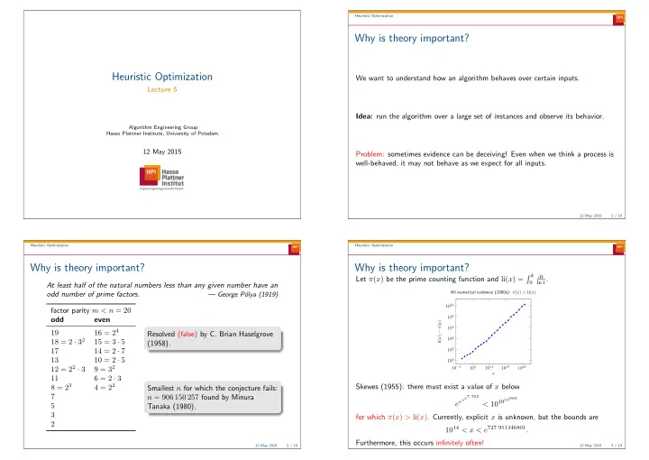
Why is theory important?

Let π(x) be the prime counting function and li(x) = k

dt ln t.

10−1 105 1011 1017 1023 100 102 104 106 108 1010 x li(x) − π(x) All numerical evidence (1900s): π(x) < li(x)

Skewes (1955): there must exist a value of x below eeee7.705 < 101010963 for which π(x) > li(x). Currently, explicit x is unknown, but the bounds are 1014 < x < e727.951346801. Furthermore, this occurs infinitely often!

12 May 2015 3 / 19

Heuristic Optimization

Why is theory important?

20 40 60 80 100 200 400 600 800 1,000 instance size runtime O(cn) O(nc) We want to make rigorous, indisputable arguments about the behavior of algorithms. We want to understand how the behavior generalizes to any problem size.

12 May 2015 4 / 19 Heuristic Optimization

Design and analysis of algorithms

Correctness

“does the algorithm always

• utput the correct solution?”

Complexity

“how many computational resources are required?”

12 May 2015 5 / 19 Heuristic Optimization

Design and analysis of algorithms

Randomized search heuristics

• Random local search
• Metropolis algorithm, simulated annealing
• Evolutionary algorithms, genetic algorithms
• Ant colony optimization

General-purpose: can be applied to any optimization problem Challenges:

• Unlike classical algorithms, they are not designed with their analysis in mind
• Behavior depends on a random number generator

12 May 2015 6 / 19 Heuristic Optimization

Convergence

First question: does the algorithm even find the solution?

Definition.

Let f : S → R for a finite set S. Let S ⊇ S⋆ := {x ∈ S : f(x) is optimal}. We say an algorithm converges if it finds an element of S⋆ with probability 1 and holds it forever after.

Two conditions for convergence (Rudolph, 1998)

• 1. There is a positive probability to reach any point in the search space from

any other point

• 2. The best solution is never lost (elitism)

Does the (1+1) EA converge on every function f : {0, 1}n → R? Does RLS converge on every function f : {0, 1}n → R? Can you think of how to modify RLS so that it converges?

12 May 2015 7 / 19

Heuristic Optimization

Runtime analysis

In most cases, randomized search heuristics visit the global optimum in finite time (or can be easily modified to do so) A far more important question: how long does it take? To characterize this unambiguously: count the number of “primitive steps” until a solution is visited for the first time (typically a function growing with the input size) We typically use asymptotic notation to classify the growth of such functions.

12 May 2015 8 / 19 Heuristic Optimization

Runtime analysis

Randomized search heuristics

• time to evaluate fitness function evaluation is much higher than the rest
• do not perform the same operations even if the input is the same
• do not output the same result if run twice

Given a function f : S → R, the runtime of some RSH A applied to f is a random variable Tf that counts the number of calls A makes to f until an optimal solution is first generated. We are interested in

• Estimating E(Tf), the expected runtime of A on f
• Estimating Pr(Tf ≤ t), the success probability of A after t steps on f

12 May 2015 9 / 19 Heuristic Optimization

Runtime analysis

RandomSearch

Choose x uniformly at random from S; while stopping criterion not met do Choose y uniformly at random from S; if f(y) ≥ f(x) then x ← y; end We already have the tools to analyze this! Suppose w.l.o.g., there is a unique maximum solution x⋆ ∈ S (if there are more, it can only be faster). Consider a run of the algorithm (x(0), x(1), . . .) where x(t) is the solution generated in the t-th iteration.

12 May 2015 10 / 19 Heuristic Optimization

Runtime analysis

Define the random variable Xt for t ∈ N0 as Xt =

• 1

if x(t) = x⋆,

• therwise;

So Xt has a Bernoulli distribution with parameter p = 1/|S| (see Lecture 3). Let T be the smallest t for which Xt = 1. Then T is a geometrically distributed random variable (see Lecture 3). Expected runtime: E(T) = 1/p = |S|

12 May 2015 11 / 19

Heuristic Optimization

Runtime analysis

Success probability: Pr(T ≤ k) = 1 − (1 − p)k For example, Pr(T ≤ |S|) = 1 − (1 − 1/|S|)|S| ≥ 1 − 1/e ≈ 0.6321 Constant chance that it takes |S| steps to find the solution. Let S = {0, 1}n. Let’s bound the success probability before 2ǫn for some constant 0 < ǫ < 1. Pr(T ≤ 2ǫn) = 1 − (1 − 2−n)2ǫn ≤ 1 − (1 − 2−n2ǫn)

• = 2−n(1−ǫ) = 2−Θ(n)

see HW 2, Exercise 2a

So the probability that random search is successful before 2Θ(n) steps is vanishing quickly (faster than every polynomial) as n grows.

12 May 2015 12 / 19 Heuristic Optimization

Runtime analysis

Let’s consider more interesting cases. . . Recall from Project 1:

(1+1) EA

Choose x uniformly at random from {0, 1}n; while stopping criterion not met do y ← x; foreach i ∈ {1, . . . , n} do With probability 1/n, yi ← (1 − yi); end if f(y) ≥ f(x) then x ← y; end In each iterations, how many bits flip in expectation? What is the probability exactly one bit flips? What is the probability exactly two bits flip? What is the probability that no bits flip?

12 May 2015 13 / 19 Heuristic Optimization

Runtime Analysis

Theorem (Droste et al., 2002)

The expected runtime of the (1+1) EA for an arbitrary function f : {0, 1}n → R is O(nn). Proof. Without loss of generality, suppose x⋆ is the unique optimum and x is the current solution. Let k = |{i : xi = x⋆

i }|.

Each bit flips (resp., does not flip) with probability 1/n (resp., with probability 1 − 1/n).

12 May 2015 14 / 19 Heuristic Optimization

Runtime Analysis

In order to reach the global optimum in the next step the algorithm has to mutate the k bits and leave the n − k bits alone. The probability to create the global optimum in the next step is 1 n k 1 − 1 n n−k ≥ 1 n n = n−n. Assuming the process has not already generated the optimal solution, in expectation we wait O(nn) steps until this happens. Note: we are simply overestimating the time to find the optimal for any arbitrary pseudo-Boolean function. Note: The upper bound is worse than for RandomSearch. In fact, there are functions where RandomSearch is guaranteed to perform better than the (1+1) EA.

12 May 2015 15 / 19

Heuristic Optimization

Initialization

Recall from Project 1: OneMax: {0, 1}n → R, x → |x|; How good is the initial solution? Let X count the number of 1-bits in the initial solution. E(X) = n/2. How likely to get exactly n/2? Pr(X = n/2) = n n/2 1 2n/2

• 1 − 1

n n/2 For n = 100, Pr(X = 50) ≈ 0.0796

12 May 2015 16 / 19 Heuristic Optimization

Initialization (Tail Inequalities)

How likely is the initial solution no worse than (3/4)n?

Markov’s Inequality

Let X be a random variable with P(X < 0) = 0. For all a > 0 we have Pr(X ≥ a) ≤ E(X) a . E(X) = n/2; then Pr(X ≥ (3/4)n) ≤ E(X) (3/4)n ≤ 2/3

12 May 2015 17 / 19 Heuristic Optimization

Initialization (Tail Inequalities)

Let X1, X2, . . . Xn be independent Poisson trials each with probability pi; For X = n

i=1 Xi, the expectation is E(X) = pi i=1.

Chernoff Bounds

• for 0 ≤ δ ≤ 1, Pr(X ≤ (1 − δ)E(X)) ≤ e

−E(x)δ2 2

.

• for δ > 0, Pr(X > (1 + δ)E(X)) ≤
• eδ

(1+δ)(1+δ)

E(X) . E.g., pi = 1/2, E(X) = n/2, fix δ = 1/2 → (1 + δ)E(X) = (3/4)n, Pr(X > (3/4)n) ≤

• e1/2

(3/2)(3/2) n/2 = c−n/2.

12 May 2015 18 / 19 Heuristic Optimization

Initialization (Tail Inequalities):

A simple example

Let n = 100. How likely is the initial solution no worse than OneMax(x) = 75? Pr(Xi) = 1/2 and E(X) = 100/2 = 50. Markov: Pr(X ≥ 75) ≤ 50

75 = 2 3.

Chernoff: Pr(X ≥ (1 + 1/2)50) ≤

• √e

(3/2)(3/2)

50 < 0.0054. In reality, Pr(X ≥ 75) = 100

i=75

100

i

• 2−100 ≈ 0.0000002818141.

12 May 2015 19 / 19