What is this talk about? Applied Asymptotics in R an R package - PowerPoint PPT Presentation

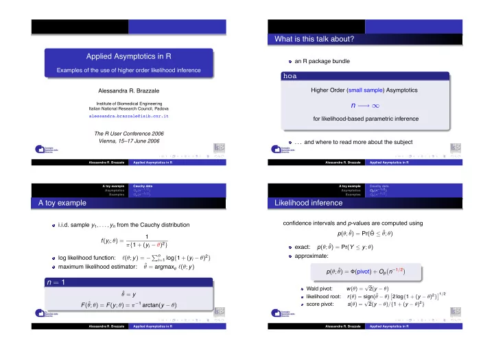
What is this talk about? Applied Asymptotics in R an R package bundle Examples of the use of higher order likelihood inference hoa Higher Order (small sample) Asymptotics Alessandra R. Brazzale Institute of Biomedical Engineering n − → ∞ Italian National Research Council, Padova alessandra.brazzale@isib.cnr.it for likelihood-based parametric inference The R User Conference 2006 Vienna, 15–17 June 2006 . . . and where to read more about the subject Alessandra R. Brazzale Applied Asymptotics in R Alessandra R. Brazzale Applied Asymptotics in R A toy example Cauchy data A toy example Cauchy data O p ( n − 1 / 2 ) O p ( n − 1 / 2 ) Asymptotics Asymptotics O p ( n − 3 / 2 ) O p ( n − 3 / 2 ) Examples Examples A toy example Likelihood inference confidence intervals and p -values are computed using i.i.d. sample y 1 , . . . , y n from the Cauchy distribution p ( θ ; ˆ θ ) = Pr (ˆ Θ ≤ ˆ θ ; θ ) 1 f ( y i ; θ ) = π { 1 + ( y i − θ ) 2 } p ( θ ; ˆ exact: θ ) = Pr ( Y ≤ y ; θ ) approximate: ℓ ( θ ; y ) = − � n i = 1 log { 1 + ( y i − θ ) 2 } log likelihood function: ˆ maximum likelihood estimator: θ = argmax θ ℓ ( θ ; y ) p ( θ ; ˆ n − 1 / 2 � � θ ) = Φ ( pivot ) + O p n = 1 √ Wald pivot: w ( θ ) = 2 ( y − θ ) ˆ θ = y � 1 / 2 r ( θ ) = sign (ˆ 2 log { 1 + ( y − θ ) 2 } likelihood root: θ − θ ) � √ θ ; θ ) = F ( y ; θ ) = π − 1 arctan ( y − θ ) F (ˆ 2 ( y − θ ) / { 1 + ( y − θ ) 2 } score pivot: s ( θ ) = Alessandra R. Brazzale Applied Asymptotics in R Alessandra R. Brazzale Applied Asymptotics in R

A toy example Cauchy data A toy example Cauchy data O p ( n − 1 / 2 ) O p ( n − 1 / 2 ) Asymptotics Asymptotics O p ( n − 3 / 2 ) O p ( n − 3 / 2 ) Examples Examples Can we do better? y = 1 . 32 ( n = 1) 1.0 p ( θ ; ˆ n − 3 / 2 � � θ ) = Φ ( pivot ) + O p significance function 0.8 0.6 modified likelihood root 0.4 r ( θ ) log s ( θ ) 1 r ∗ ( θ ) = r ( θ ) + 0.2 r ( θ ) 0.0 � 4 � 2 0 2 4 � � Alessandra R. Brazzale Applied Asymptotics in R Alessandra R. Brazzale Applied Asymptotics in R A toy example Cauchy data A toy example First order O p ( n − 1 / 2 ) Asymptotics Asymptotics Higher order O p ( n − 3 / 2 ) Examples Examples in R And what if n > 1? General theory There is no exact solution, but . . . θ = ( ψ , λ ) , with scalar parameter of interest ψ significance function marg[hoa] package p ( ψ ; ˆ ψ ) = Pr (ˆ Ψ ≤ ˆ ψ ; ψ ) > library( marg ) ℓ p ( ψ ) = ℓ ( ψ , ˆ > set.seed( 321 ) profile log likelihood: λ ψ ; y ) > y <- rt( n = 15, df = 3 ) w ( θ ) = j p ( ˆ ψ ) 1 / 2 ( ˆ > y.rsm <- rsm( y ~ 1, family = student(3) ) Wald statistic: ψ − ψ ) � 1 / 2 > y.cond <- cond( y.rsm, offset = 1 ) � r ( θ ) = sign ( ˆ 2 { ℓ p ( ˆ likelihood root: ψ − ψ ) ψ ) − ℓ p ( ψ ) } > summary( y.cond, test = 0 ) s ( θ ) = j p ( ˆ ψ ) − 1 / 2 d ℓ p ( ψ ) / d ψ score statistic: with j p ( ψ ) = − d 2 ℓ p ( ψ ) / d ψ 2 0.354 ( r ∗ ) p -values: 0.282 (Wald), 0.306 ( r ), Alessandra R. Brazzale Applied Asymptotics in R Alessandra R. Brazzale Applied Asymptotics in R

A toy example First order A toy example First order Asymptotics Higher order Asymptotics Higher order Examples in R Examples in R Higher order inference The hoa bundle cond : logistic regression Modified likelihood root exp ( x ⊤ i β ) r ( ψ ) log q ( ψ ) 1 Pr ( Y i = 1 ; β ) = r ∗ ( ψ ) = r ( ψ ) + 1 + exp ( x ⊤ i β ) r ( ψ ) marg : linear nonnormal models with q ( ψ ) representing a suitable correction term y i = x ⊤ i β + σε i , ε i ∼ f 0 ( · ) p ( ψ ; ˆ ψ ) = Φ { r ∗ ( ψ ) } + O p ( n − 3 / 2 ) nlreg : nonlinear heteroscedastic regression r ∗ ( ψ ) = r ( ψ ) + r inf ( ψ ) + r np ( ψ ) y ij = µ ( x i ; β ) + ω ( x i ; β , ρ ) ε ij , ε ij ∼ N ( 0 , 1 ) r inf ( ψ ) : information adjustment r np ( ψ ) : nuisance parameter adjustment csampling : conditional sampling routines Alessandra R. Brazzale Applied Asymptotics in R Alessandra R. Brazzale Applied Asymptotics in R A toy example A toy example Logistic regression Logistic regression Asymptotics Asymptotics Nonlinear regression Nonlinear regression Examples Examples airway data airway data (2/3) > head(airway) > airway.glm <- glm( formula(airway), family = binomial, response age sex lubricant duration type + data = airway ) 1 0 48 1 0 45 0 > library( cond ) 2 0 48 1 0 15 0 3 1 39 0 1 40 0 > airway.cond <- cond( airway.glm, offset = type1 ) 4 1 59 1 0 83 1 5 1 24 1 1 90 1 > summary( airway.cond ) 6 1 55 1 1 25 1 Collet (1998) Alessandra R. Brazzale Applied Asymptotics in R Alessandra R. Brazzale Applied Asymptotics in R

A toy example A toy example Logistic regression Logistic regression Asymptotics Asymptotics Nonlinear regression Nonlinear regression Examples Examples airway data (3/3) calcium uptake data > library( boot) Confidence intervals -------------------- > head( calcium ) level = 95 % lower two-sided upper time cal Wald pivot -3.486 0.2271 1 0.45 0.34170 Wald pivot (cond. MLE) -3.053 0.2655 Likelihood root -3.682 0.1542 2 0.45 -0.00438 Modified lik. root -3.130 0.2558 3 0.45 0.82531 Modified lik. (cont. corr.) -3.592 0.5649 4 1.30 1.77967 5 1.30 0.95384 Diagnostics: 6 1.30 0.64080 ----------- INF NP Davison & Hinkley (1997, Example 7.7) 0.05855 0.51426 Alessandra R. Brazzale Applied Asymptotics in R Alessandra R. Brazzale Applied Asymptotics in R A toy example A toy example Logistic regression Logistic regression Asymptotics Asymptotics Nonlinear regression Nonlinear regression Examples Examples calcium uptake data (2/3) b0 3 3 3 3 2 2 2 2 1 1 1 1 0 0 0 0 � 1 � 1 � 1 � 1 � 2 � 2 � 2 � 2 � 3 � 3 � 3 � 3 1 + x γ � 4 ω 2 ( x i ; γ ) = σ 2 � � µ ( x i ; β ) = β 0 { 1 − exp ( − β 1 x i ) } , i 3.5 4.5 5.5 � 3 0 2 � 3 0 2 � 3 0 2 b1 0.35 3 3 3 2 2 2 0.30 > library( nlreg ) 1 1 1 0.25 0 0 0 � 1 0.20 � 1 � 1 � 2 0.15 � 2 � 2 � 3 0.10 � 3 � 3 � 4 > calcium.nl <- 3.5 4.5 5.5 0.15 0.30 � 3 0 2 � 3 0 2 + nlreg( cal ~ b0 * (1 - exp(-b1 * time)), g + weights = ~ 1 + time^g, data = calcium, 1.5 1.5 3 3 2 1.0 1.0 2 � � 1 1 + start = c(b0 = 4, b1 = 0.1, g = 0) ) 0.5 0.5 0 0 0.0 0.0 � 1 � 1 � 0.5 � 0.5 � 2 � � 2 � 1.0 � 1.0 � 3 � � 3 � 4 > calcium.prof <- profile( calcium.nl ) 3.5 4.5 5.5 0.10 0.25 � 1.0 0.5 � 3 0 2 logs � 0.5 � 0.5 � 0.5 3 > contour( calcium.prof, alpha = 0.05, lwd1 = 2, � 1.0 � 1.0 � 1.0 � 2 � 1.5 � 1.5 � 1.5 � 1 � 2.0 � 2.0 � 2.0 + lwd2 = 2 ) 0 � 2.5 � 2.5 � 2.5 � 1 � 3.0 � 3.0 � 3.0 � 2 � 3.5 � 3.5 � 3.5 � � � 3 � 4.0 � 4.0 � 4.0 3.5 4.5 5.5 0.10 0.25 � 1.5 0.0 1.5 � 3.5 � 1.5 Alessandra R. Brazzale Applied Asymptotics in R Alessandra R. Brazzale Applied Asymptotics in R

Applied Asymptotics Applied Asymptotics To wind up To wind up Credits Credits And if you wish to try more . . . Credits Brazzale, A. R. (2005). hoa: An R package bundle for higher order likelihood inference. Rnews , Vol. 5/1, May 2005, pp. 20–27. Alessandra Salvan, Anthony C. Davison, Nancy Reid R vignette in hoa v. 1.1-0 Ruggero Bellio Douglas M. Bates, Kurt Hornik, Torsten Hothorn Brazzale, A. R., Davison, A. C. and Reid, N. (2006). Applied Asymptotics . Cambridge University Press. . . . and the useRs! (Forthcoming) www.isib.cnr.it/ ∼ brazzale/CS theory & implementation & examples and case studies Alessandra R. Brazzale Applied Asymptotics in R Alessandra R. Brazzale Applied Asymptotics in R