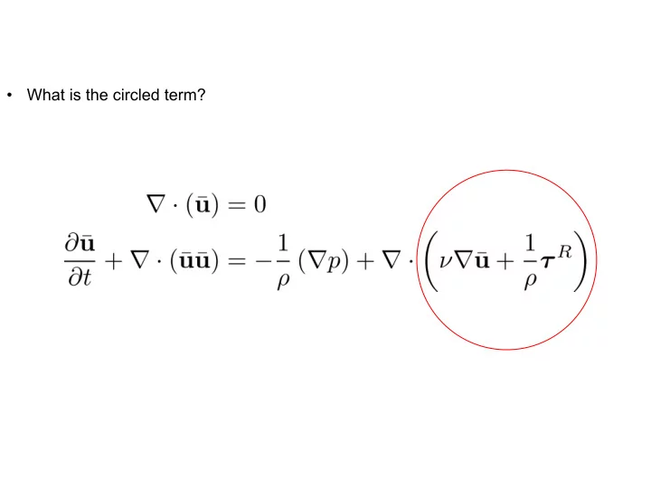
What is the circled term? The circled term represents the total - PowerPoint PPT Presentation

• What is the circled term?

• The circled term represents the total stresses, • The total stresses can be decomposed in a laminar contribution and a turbulent contribution. • Where each contribution is given by,

• The laminar (or viscous) stresses can be computed from the molecular viscosity and the mean velocity gradient, • The turbulent stresses (Reynolds stresses), can be computed as follows, • As we have seen, this term is a little bit trickier to compute. • This term can be approximated or modeled ( e.g. , by using the Boussinesq approximation). • Or it can be resolved (DNS, LES, DES, experiments).

• We can approximate the Reynolds stresses by using the Boussinesq approximation, • Or we can directly resolve it, • We can derive a transport equation for each term of the Reynolds stress tensor , or we can resolve the velocity fluctuations using SRS simulations (DES, LES, DNS).

• If we make the assumptions that we are working with a 2D boundary layer, the total stress can be approximated as follows, • With no simplifications (3D case), the total shear stress is computed as follows,

• Statistical moments. Mean Variance Skewness Kurtosis

• In lecture 5, we talked about first order and second order closure methods. • Let us recall these methods. • In analogy to the statistical moments, • First order closure methods (or first moment closure), approximate the solution using the mean velocity field. • They are based on the Boussinesq approximation, • Second order closure methods (or second moment closure), compute the solution using the mean turbulent field, • Where

• Second order closure methods are based on the Reynolds stress equations, • The previous equations can be rewritten as,

• There are higher order closure methods. • For example, the equations for the third order moments, read as, • Notice that we keep multiplying by the mean fluctuating velocity (in analogy to the statistical moments).

• Recall that the turbulent kinetic energy can be computed as follows, • If you are running SRS simulations, you need to compute the average of the product of the fluctuations. • The product of the fluctuations are derived from the primitive variables. • Therefore, before running, remember to set the unsteady statistics and define the products of the fluctuating quantities. Instantaneous field Mean field

• To stress this point. • All the correlations (or products) appearing in the Reynolds stress tensor, are computed from the instantaneous field. • Therefore, you need to compute the unsteady statistics and define these variables, that is, the products of the fluctuations. • Recall that the Reynolds stress tensor read as,

• Two-point correlation. x + r x Two-point velocity correlation tensor Autocorrelation tensor

• Two-point correlation. Longitudinal velocity correlation coefficient Lateral velocity correlation coefficient Longitudinal length scale Lateral length scale

• Time series of the measured stream wise and wall-normal velocity components measured by means of laser-Doppler velocimetry. • Left image. Time series of the measured stream wise (u component) and wall-normal (v component) velocity measured by means of laser-Doppler velocimetry in a turbulent boundary layer over a flat plate • Right image. The correlation of the fluctuations u’ = u − u and v’ = v − v. The ellipse represents the correlation between the two velocity components, i.e. u’v’, or Reynolds stress. The main axes of the ellipse are proportional to σ u and σ v , respectively. The measurement was taken at a distance of y + = 20 viscous wall-units from the plate. • Images adapted from reference [1]. [1] F. Nieuwstadt, B. Boersma, J. Westerweel. Turbulence. Introduction to Theory and Applications of Turbulent Flows. Springer, 2016.

• The turbulence intensity is defined as follows, • Where RMS stands for root mean square. • The RMS of the velocity is equivalent to the velocity fluctuations, • The standard deviation is the same as the root mean squared, if it is defined about zero. • We use the RMS to compute the turbulent intensity because otherwise you will get turbulent intensity levels that are too high. • When you see the quantity RMS in solvers, it means that the fluctuations are computed about zero.

• The normal Reynolds stresses can be normalized relative to the mean flow velocity, as follows, • These three quantities are known as relative intensities. Turbulence intensities for a flat-plate boundary layer of thickness [1]. [1] P. Klebanoff. “Characteristics of Turbulence in a Boundary Layer with Zero Pressure Gradient”. NACA TN 1247, 1955.