What is a What are Support Vector Machines Support Vector Machine? - - PDF document

SLIDE 1

1

CS 540, University of Wisconsin-Madison, C. R. Dyer

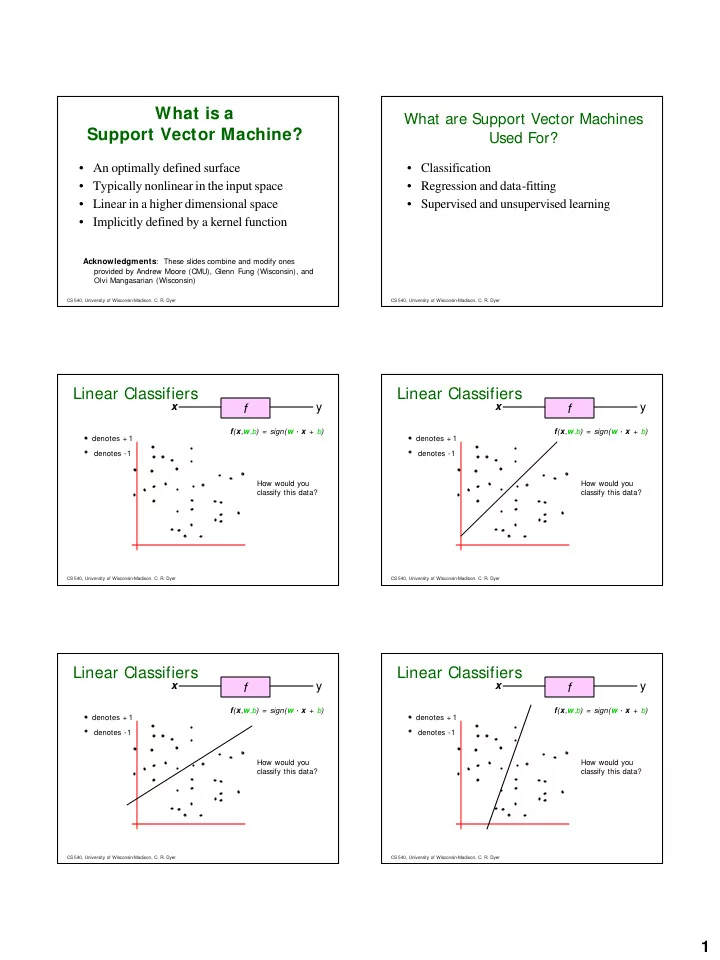
What is a Support Vector Machine?

• An optimally defined surface
• Typically nonlinear in the input space
• Linear in a higher dimensional space
• Implicitly defined by a kernel function

Acknowledgments: These slides combine and modify ones provided by Andrew Moore (CMU), Glenn Fung (Wisconsin), and Olvi Mangasarian (Wisconsin)

CS 540, University of Wisconsin-Madison, C. R. Dyer

What are Support Vector Machines Used For?

• Classification
• Regression and data-fitting
• Supervised and unsupervised learning

CS 540, University of Wisconsin-Madison, C. R. Dyer

Linear Classifiers

f

x

y

denotes + 1 denotes -1 f(x,w,b) = sign(w · x + b) How would you classify this data?

CS 540, University of Wisconsin-Madison, C. R. Dyer

Linear Classifiers

f

x

y

denotes + 1 denotes -1 f(x,w,b) = sign(w · x + b) How would you classify this data?

CS 540, University of Wisconsin-Madison, C. R. Dyer

Linear Classifiers

f

x

y

denotes + 1 denotes -1 f(x,w,b) = sign(w · x + b) How would you classify this data?

CS 540, University of Wisconsin-Madison, C. R. Dyer

Linear Classifiers

f

x

y

denotes + 1 denotes -1 f(x,w,b) = sign(w · x + b) How would you classify this data?

SLIDE 2

2

CS 540, University of Wisconsin-Madison, C. R. Dyer

Linear Classifiers

f

x

y

denotes + 1 denotes -1 f(x,w,b) = sign(w · x + b) Any of these would be fine … … but which is best?

CS 540, University of Wisconsin-Madison, C. R. Dyer

Classifier Margin

f

x

y

denotes + 1 denotes -1 f(x,w,b) = sign(w · x + b)

Define the margin

• f a linear

classifier as the width that the boundary could be increased by before hitting a data point

CS 540, University of Wisconsin-Madison, C. R. Dyer

Maximum Margin

f

x

y

denotes + 1 denotes -1 f(x,w,b) = sign(w · x + b)

The maximum margin linear classifier is the linear classifier with the, um, maximum margin. This is the simplest kind of SVM (Called an LSVM)

Linear SVM

CS 540, University of Wisconsin-Madison, C. R. Dyer

Maximum Margin

f

x

y

denotes + 1 denotes -1 f(x,w,b) = sign(w · x + b)

The maximum margin linear classifier is the linear classifier with the, um, maximum margin. This is the simplest kind of SVM (Called an LSVM)

Support Vectors are those data points that the margin pushes up against # SV's < < # DP Linear SVM

CS 540, University of Wisconsin-Madison, C. R. Dyer

Why Maximum Margin?

denotes + 1 denotes -1 f(x,w,b) = sign(w. x - b)

The maximum margin linear classifier is the linear classifier with the, um, maximum margin. This is the simplest kind of SVM (Called an LSVM)

1. Intuitively this feels safest 2. If we’ve made a small error in the location of the boundary (it’s been jolted in its perpendicular direction) this gives us least chance of causing a misclassification 3. Robust to outliers since the model is immune to change/removal of any non-support-vector data points 4. There’s some theory that is related to (but not the same as) the proposition that this is a good thing 5. Empirically it works very well Support Vectors are those data points that the margin pushes up against # SV's < < # DP

CS 540, University of Wisconsin-Madison, C. R. Dyer

Specifying a Line and Margin

• How do we represent this mathematically?
• …

in m input dimensions?

Plus-Plane Minus-Plane Classifier Boundary “Predict C lass = +1” zone “Predict Class =

• 1”

zone

SLIDE 3

3

CS 540, University of Wisconsin-Madison, C. R. Dyer

Specifying a Line and Margin

• Plus-plane = { w · x + b = + 1 }
• Minus-plane = { w · x + b = -1 }

Plus-Plane Minus-Plane Classifier Boundary “Predict C lass = +1” zone “Predict Class =

• 1”

zone

• 1 < w · x + b < 1

if Universe explodes w · x + b = -1 if

• 1

i.e. sign() w · x + b ≥ 1 if + 1 Classify as..

wx+ b= 1 wx+ b= 0 wx+b= -1 CS 540, University of Wisconsin-Madison, C. R. Dyer

Computing the Margin

• Plus-plane = { w x + b = + 1 }
• Minus-plane = { w x + b = -1 }
• The vector w is perpendicular to the Plus Plane

“Predict C lass = +1” zone “Predict Class =

• 1”

zone

wx+ b= 1 wx+ b= 0 wx+b= -1

M = Margin (width)

How do we compute M in terms of w and b?

w

CS 540, University of Wisconsin-Madison, C. R. Dyer

Computing the Margin

• Plus-plane = { w x + b = + 1 }
• Minus-plane = { w x + b = -1 }
• The vector w is perpendicular to the Plus Plane
• Let x - be any point on the minus plane
• Let x + be the closest plus-plane-point to x -

“Predict C lass = +1” zone “Predict Class =

• 1”

zone

wx+ b= 1 wx+ b= 0 wx+b= -1

M = Margin

How do we compute M in terms of w and b?

x- x+

Any location in m: not necessarily a datapoint Any location in Rm: not necessarily a data point

w

CS 540, University of Wisconsin-Madison, C. R. Dyer

Computing the Margin

• Plus-plane = { w x + b = + 1 }
• Minus-plane = { w x + b = -1 }
• The vector w is perpendicular to the Plus Plane
• Let x - be any point on the minus plane
• Let x + be the closest plus-plane-point to x -
• Claim : x + = x - + λ w

for some value of λ. Why?

“Predict C lass = +1” zone “Predict Class =

• 1”

zone

wx+ b= 1 wx+ b= 0 wx+b= -1

M = Margin

How do we compute M in terms of w and b?

x- x+ w

CS 540, University of Wisconsin-Madison, C. R. Dyer

Computing the Margin

• Plus-plane = { w x + b = + 1 }
• Minus-plane = { w x + b = -1 }
• The vector w is perpendicular to the Plus Plane
• Let x - be any point on the minus plane
• Let x + be the closest plus-plane-point to x -
• Claim : x + = x - + λ w

for some value of λ. Why?

“Predict C lass = +1” zone “Predict Class =

• 1”

zone

wx+ b= 1 wx+ b= 0 wx+b= -1

M = Margin

How do we compute M in terms of w and b?

x- x+ The line from x - to x + is perpendicular to the planes So to get from x - to x + travel some distance in direction w w

CS 540, University of Wisconsin-Madison, C. R. Dyer

Computing the Margin

What we know:

• w x + + b = + 1
• w x - + b = -1
• x + = x - + λ w
• | x + - x - | = M

It’s now easy to get M in terms of w and b

“Predict C lass = +1” zone “Predict Class =

• 1”

zone

wx+ b= 1 wx+ b= 0 wx+b= -1

M = Margin x- x+ w

SLIDE 4

4

CS 540, University of Wisconsin-Madison, C. R. Dyer

Computing the Margin

What we know:

• w x + + b = + 1
• w x - + b = -1
• x + = x - + λ w
• | x + - x - | = M

It’s now easy to get M in terms of w and b

“Predict C lass = +1” zone “Predict Class =

• 1”

zone

wx+ b= 1 wx+ b= 0 wx+b= -1

M = Margin

w (x - + λ w) + b = 1 ⇒ w x - + b + λ ww = 1 ⇒

• 1 + λ ww = 1

⇒ x- x+

w.w 2 = ?

w

CS 540, University of Wisconsin-Madison, C. R. Dyer

Computing the Margin

w.w 2 = ?

“Predict C lass = +1” zone “Predict Class =

• 1”

zone

wx+ b= 1 wx+ b= 0 wx+b= -1

M = Margin = M = | x + - x- | = | λ w | = x- x+

w w w w w w . 2 . . 2 = = w w w . | | ? ? = =

w w. 2

w What we know:

• w x + + b = + 1
• w x - + b = -1
• x + = x - + λ w
• | x + - x - | = M

It’s now easy to get M in terms of w and b

CS 540, University of Wisconsin-Madison, C. R. Dyer

Learning the Maximum Margin Classifier

Given a guess of w and b we can

• Compute whether all data points in the correct half -planes
• Compute the width of the margin

So now we just need to write a program to search the space

• f w’s and b’s to find the widest margin that matches all

the data points. How ?

“Predict C lass = +1” zone “Predict Class =

• 1”

zone

wx+ b= 1 wx+ b= 0 wx+b= -1

M = Margin = x- x+ w w. 2 w

CS 540, University of Wisconsin-Madison, C. R. Dyer

Learning via Quadratic Programming

• QP is a well-studied class of optimization

algorithms to maximize a quadratic function of some real-valued variables subject to linear constraints

CS 540, University of Wisconsin-Madison, C. R. Dyer

Uh-oh!

denotes + 1 denotes -1

This is going to be a problem! What should we do?

CS 540, University of Wisconsin-Madison, C. R. Dyer

Uh-oh!

denotes + 1 denotes -1

This is going to be a problem! What should we do? Idea: Minimize ||w|| 2 + C (distance of error points to their correct place)

SLIDE 5

5

CS 540, University of Wisconsin-Madison, C. R. Dyer

An Equivalent QP

Maximize

∑∑ ∑

= = =

+

R k R l kl l k R k k

Q a a a

1 1 1

where

) . (

l k l k kl

y y Q x x =

Subject to these constraints:

k C a k ∀ ≤ ≤

Then define:

∑

=

=

R k k k k y

a

1

x w

k k K K K K

a K e y b max arg where . ) 1 ( = − − = w x

Then classify with: f(x,w,b) = sign(w. x - b)

1

=

∑

= R k k k y

a

CS 540, University of Wisconsin-Madison, C. R. Dyer

An Equivalent QP

Maximize

∑∑ ∑

= = =

+

R k R l kl l k R k k

Q a a a

1 1 1

where

) . (

l k l k kl

y y Q x x =

Subject to these constraints:

k C a k ∀ ≤ ≤

Then define:

∑

=

=

R k k k k y

a

1

x w

k k K K K K

a K e y b max arg where . ) 1 ( = − − = w x

Then classify with: f(x,w,b) = sign(w. x - b)

1

=

∑

= R k k k y

a

αk associated with data point are 0 except for support vectors ..so this sum only needs to be over the support vectors. Has only a single global maximum which can be found efficiently Data enter the expression as dot product of pairs or points

CS 540, University of Wisconsin-Madison, C. R. Dyer

Suppose we’re in 1 Dimension

What would SVMs do with this data?

x= 0

CS 540, University of Wisconsin-Madison, C. R. Dyer

Suppose we’re in 1 Dimension

Not a big surprise

Positive “plane” Negative “plane”

x= 0

CS 540, University of Wisconsin-Madison, C. R. Dyer

Harder 1-Dimensional Dataset

Not as easy! What can be done about this?

x= 0

CS 540, University of Wisconsin-Madison, C. R. Dyer

Harder 1-Dimensional Dataset

x= 0

) , (

2 k k k

x x = z

The Kernel Trick: Preprocess the data, mapping x into higher dimensional space F(x)

SLIDE 6

6

CS 540, University of Wisconsin-Madison, C. R. Dyer

Harder 1-Dimensional Dataset

x= 0

) , (

2 k k k

x x = z

The Kernel Trick: Preprocess the data, mapping x into higher dimensional space F(x)

CS 540, University of Wisconsin-Madison, C. R. Dyer CS 540, University of Wisconsin-Madison, C. R. Dyer

• Project examples into some higher dimensional space

where the data is linearly separable, defined by z = F(x)

• Training depends only on dot products of the form

F(xi) · F(xj)

• Example:

K(xi, xj) = F(xi) · F(xj) = (xi · xj)2

) , 2 , ( ) (

2 2 2 1 2 1

x x x x x F =

Maximize

∑∑ ∑

= = =

+

R k R l kl l k R k k

Q a a a

1 1 1

where

) . (

l k l k kl

y y Q x x =

CS 540, University of Wisconsin-Madison, C. R. Dyer

Common SVM Basis Functions

zk = ( polynomial terms of xk of degree 1 to q ) zk = ( radial basis functions of xk ) zk = ( sigmoid functions of xk )

        − = = KW | | KernelFn ) ( ] [

j k k j k

f j c x x z

CS 540, University of Wisconsin-Madison, C. R. Dyer

SVM Kernel Functions

• K(a,b)= (a . b + 1)d is an example of an SVM

kernel function

• Beyond polynomials there are other very high

dimensional basis functions that can be made practical by finding the right kernel function

• Radial-Basis-style Kernel Function:
• Neural-Net-style Kernel Function:

        − − =

2 2

2 ) ( exp ) , ( σ b a b a K ) . tanh( ) , ( δ κ − = b a b a K

σ, κ and δ are magic parameters that must be chosen by a model selection method such as CV or VCSRM

CS 540, University of Wisconsin-Madison, C. R. Dyer

The Federalist Papers

• Written in 1787-1788 by Alexander Hamilton,

John Jay, and James Madison to persuade the citizens of New York to ratify the constitution

• Papers consisted of short essays, 900 to 3500 words

in length

• Authorship of 12 of those papers have been in

dispute ( Madison or Hamilton); these papers are referred to as the disputed Federalist papers

SLIDE 7

7

CS 540, University of Wisconsin-Madison, C. R. Dyer

Description of the Data

• For every paper:
• Machine readable text was created using a scanner
• Computed relative frequencies of 70 words that

Mosteller-Wallace identified as good candidates for author-attribution studies

• Each document is represented as a vector containing the

70 real numbers corresponding to the 70 word frequencies

• The dataset consists of 118 papers:
• 50 Madison papers
• 56 Hamilton papers
• 12 disputed papers

CS 540, University of Wisconsin-Madison, C. R. Dyer

Function Words Based on Relative Frequencies

CS 540, University of Wisconsin-Madison, C. R. Dyer

SLA Feature Selection for Classifying the Disputed Federalist Papers

• Apply the SVM Successive Linearization

Algorithm for feature selection to:

• Train on the 106 Federalist papers with known

authors

• Find a classification hyperplanethat uses as few

words as possible

• Use the hyperplane to classify the 12

disputed papers

CS 540, University of Wisconsin-Madison, C. R. Dyer

Hyperplane Classifier Using 3 Words

• A hyperplane depending on three words

was found:

0.537to + 24.663upon + 2.953would = 66.616

• All disputed papers ended up on the

Madison side of the plane

CS 540, University of Wisconsin-Madison, C. R. Dyer

Results: 3D Plot of Hyperplane

CS 540, University of Wisconsin-Madison, C. R. Dyer

Multi-Class Classification

• SVMs can only handle two-class outputs
• What can be done?
• Answer: for N-class problems, learn N SVM’s:
• SVM 1 learns “Output= 1” v s “Output ≠ 1”
• SVM 2 learns “Output= 2” v s “Output ≠ 2”
• :
• SVM N learns “Output= N” v s “Output ≠ N”
• To predict the output for a new input, just predict

with each SVM and find out which one puts the prediction the furthest into the positive region

SLIDE 8

8

CS 540, University of Wisconsin-Madison, C. R. Dyer

Summary

• Learning linear functions
• Pick separating plane that maximizes margin
• Separating plane defined in terms of support

vectors only

• Learning non-linear functions
• Project data into higher dimensional space
• Use kernel functions for efficiency
• Generally avoids over-fitting problem
• Global optimization method; no local optima
• Can be expensive to apply, especially for multi-

class problems