Welcome back. Edge Expansion/Conductance. Spectra of the graph. - PowerPoint PPT Presentation

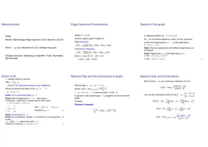
Welcome back. Edge Expansion/Conductance. Spectra of the graph. Graph G = ( V , E ) , A : Adjacency Matrix A ij = 1 ⇔ ( i , j ) ∈ E Today. Assume regular graph of degree d . M = 1 d A , normalized adjacency matrix, M real, symmetric Review: Spectral gap, Edge expansion h ( G ) , Sparsity φ ( G ) etc. Edge Expansion. orthonormal eigenvectors: v 1 ,..., v n with eigenvalues | E ( S , V − S ) | λ 1 ≥ λ 2 ≥ ... ≥ λ n h ( S ) = d min ( | S | , | V − S | ) , h ( G ) = min S ⊂ V h ( S ) Write 1 − λ 2 as a relaxation of φ ( G ) , Cheeger easy part Claim: Any two eigenvectors with different eigenvalues are Conductance (Sparsity). orthogonal. φ ( S ) = n | E ( S , V − S ) | d | S || V − S | , φ ( G ) = min S ⊂ V φ ( S ) Proof: Eigenvectors: v , v ′ with eigenvalues λ , λ ′ . v T Mv ′ = v T ( λ ′ v ′ ) = λ ′ v T v ′ Cheeger hard part: Sweeping cut Algorithm, Proof, Asymptotic Note n ≥ max ( | S | , | V |−| S | ) ≥ n / 2 tight example v T Mv ′ = λ v T v ′ = λ v T v . → h ( G ) ≤ φ ( G ) ≤ 2 h ( S ) Action of M . Spectral Gap and the connectivity of graph. Spectral Gap and Conductance. v - assigns values to vertices. We will show 1 − λ 2 as a continuous relaxation of φ ( G ) . ( Mv ) i = 1 d ∑ j ∼ i v j . Spectral gap: µ = λ 1 − λ 2 = 1 − λ 2 . Action of M : taking the average of your neighbours. n | E ( S , V − S ) | φ ( G ) = min S ∈ V | E ( S , V − S ) | (Direct) result from the action of M , | λ i | ≤ 1 ∀ i d | S || V − S | Recall: h ( G ) = min S , | S |≤| V | / 2 | S | v 1 = 1 . λ 1 = 1. 1 − λ 2 = 0 ⇔ λ 2 = 1 ⇔ G disconnected ⇔ h ( G ) = 0 � 1 if i ∈ S Let x be the characteritic vector of set S x i = Claim: For a connected graph λ 2 < 1. In general, small spectral gap 1 − λ 2 suggests ”poorly connected” 0 if i �∈ S graph Proof: Second Eigenvector: v ⊥ 1 . Max value x . | E ( S , V − S ) | = 1 A ij | x i − x j | = d Connected → path from x valued node to lower value. 2 ∑ 2 ∑ M ij ( x i − x j ) 2 Formally → ∃ e = ( i , j ) , v i = x , x j < x . i , j i , j Cheeger’s Inequality j i ( Mv ) i ≤ 1 d ( x + x ··· + v j ) < x . | S || V − S | = 1 | x i − x j | = 1 . 2 ∑ 2 ∑ ( x i − x j ) 2 . 1 − λ 2 . � Therefore λ 2 < 1. ≤ h ( G ) ≤ 2 ( 1 − λ 2 ) x i , j i , j ≤ x 2 Claim: Connected if λ 2 < 1. n ∑ i , j M ij ( x i − x j ) 2 φ ( G ) = min x ∈{ 0 , 1 } V −{ 0 , 1 } Proof: By contradiction. Assign + 1 to vertices in one component, − δ ∑ i , j ( x i − x j ) 2 to rest. x i = ( Mx i ) = ⇒ eigenvector with λ = 1. Choose δ to make ∑ i x i = 0, i.e., x ⊥ 1 .

Combining the two claims, we get x T Mx Recall Rayleigh Quotient: λ 2 = max x ∈ R V −{ 0 } , x ⊥ 1 x T x x T Mx 2 ( x T x − x T Mx ) Recall Rayleigh Quotient: λ 2 = max x ∈ R V −{ 0 } , x ⊥ 1 ∑ i , j M ij ( x i − x j ) 2 x T x 1 − λ 2 = min x ∈ R V −{ 0 } , x ⊥ 1 1 − λ 2 = min x ∈ R V −{ 0 } , x ⊥ 1 2 x T x 1 n ∑ i , j ( x i − x j ) 2 2 ( x T x − x T Mx ) Claim: 2 ( x T x − x T Mx ) = ∑ i , j M ij ( x i − x j ) 2 1 − λ 2 = min x ∈ R V −{ 0 } , x ⊥ 1 ∑ i , j M ij ( x i − x j ) 2 2 x T x = min x ∈ R V − Span { 1 } n ∑ i , j ( x i − x j ) 2 1 Proof: Claim: 2 x T x = 1 n ∑ i , j ( x i − x j ) 2 M ij ( x i − x j ) 2 = ∑ M ij ( x 2 i + x 2 ∑ j ) − 2 ∑ M ij x i x j Proof: i , j i , j i , j Recall ( x i − x j ) 2 = ∑ x 2 i + x 2 1 ∑ j − 2 x i x j j ) − 2 x T Mx = ∑ d ( x 2 i + x 2 n ∑ i , j M ij ( x i − x j ) 2 i ∑ φ ( G ) = min x ∈{ 0 , 1 } V −{ 0 , 1 } i , j i , j j ∼ i ∑ i , j ( x i − x j ) 2 x i ) 2 = 2 n ∑ i = 2 nx T x x 2 x 2 = 2 n ∑ i − 2 ( ∑ 1 = 2 ∑ j ) − 2 x T Mx d ( x 2 i + x 2 i i i We have 1 − λ 2 as a continuous relaxation of φ ( G ) , thus ( i , j ) ∈ E We used x ⊥ 1 ⇒ ∑ i x i = 0 i − 2 x T Mx = 2 x T x − 2 x T Mx x 2 = 2 ∑ 1 − λ 2 ≤ φ ( G ) ≤ 2 h ( G ) i Hooray!! We get the easy part of Cheeger 1 − λ 2 ≤ h ( G ) 2 Cheeger Hard Part. Sweeping Cut Algorithm Proof of Main Lemma � Now let’s get to the hard part of Cheeger h ( G ) ≤ 2 ( 1 − λ 2 ) . WLOG V = { 1 ,..., n } x 1 ≤ x 2 ≤ ... ≤ x n Input: G = ( V , E ) , x ∈ R V , x ⊥ 1 Idea : We have 1 − λ 2 as a continuous relaxation of φ ( G ) Want to show Sort the vertices in non-decreasing order in terms of their values in x ∑ i , j M ij ( x i − x j ) 2 Take the 2 nd eigenvector x = argmin x ∈ R V − Span { 1 } WLOG V = { 1 ,..., n } x 1 ≤ x 2 ≤ ... ≤ x n 1 √ d | E ( S , V − S ) | 1 n ∑ i , j ( x i − x j ) 2 ∃ i s.t. h ( S i ) = min ( | S | , | V − S | ) ≤ 2 δ Let S i = { 1 ,..., i } i = 1 ,..., n − 1 Consider x as an embedding of the vertices to the real line. Return S = argmin S i h ( S i ) Round x to get a x ∈ { 0 , 1 } V Probabilistic Argument: Construct a distribution D over { S 1 ,..., S n − 1 } Main Lemma: G = ( V , E ) , d -regular Rounding: Take a threshold t , such that x ∈ R V , x ⊥ 1 , δ = ∑ i , j M ij ( x i − x j ) 2 E S ∼ D [ 1 √ � d | E ( S , V − S ) | ] x i ≥ t → x i = 1 n ∑ i , j ( x i − x j ) 2 1 E S ∼ D [ min ( | S | , | V − S | )] ≤ 2 δ √ x i < t → x i = 0 If S is the ouput of the sweeping cut algorithm, then h ( S ) ≤ 2 δ √ Note: Applying the Main Lemma with the 2 nd eigenvector v 2 , we have What will be a good t ? → E S ∼ D [ 1 d | E ( S , V − S ) |− 2 δ min ( | S | , | V − S | )] ≤ 0 √ � δ = 1 − λ 2 , and h ( G ) ≤ h ( S ) ≤ 2 ( 1 − λ 2 ) . Done! We don’t know. Try all possible thresholds ( n − 1 possibilities), and 1 ∃ S d | E ( S , V − S ) |− 2 δ min ( | S | , | V − S | ) ≤ 0 hope there is a t leading to a good cut!

The distribution D √ E S ∼ D [ 1 d | E ( S , V − S ) | ] √ Goal: E S ∼ D [ min ( | S | , | V − S | )] ≤ 2 δ E S ∼ D [ 1 d | E ( S , V − S ) | ] Goal: E S ∼ D [ min ( | S | , | V − S | )] ≤ 2 δ Numerator: Denominator: Let T i , j = i , j is cut by ( S , V − S ) Let T i = i is in the smaller set of S , V − S 2 ⌋ = 0, and x 2 1 + x 2 WLOG, shift and scale so that x ⌊ n n = 1 Can check � Pr [ T i , j ] = | x 2 i − x 2 x i , x j same sign: j | E S ∼ D [ T i ] = Pr [ T i ] = x 2 Take t from the range [ x 1 , x n ] with density function f ( t ) = 2 | t | . Pr [ T i , j ] = x 2 i + x 2 i x i , x j different sign: j � x n � 0 � x n 0 2 t d t = x 2 1 + x 2 Check: x 1 f ( t ) d t = x 1 − 2 t d t + n = 1 A common upper bound: E [ T i , j ] = Pr [ T i , j ] ≤ | x i − x j | ( | x i | + | x j | ) S = { i : x i ≤ t } E S ∼ D [ min ( | S | , | V − S | )] = E S ∼ D [ ∑ T i ] i Take D as the distribution over S 1 ,..., S n − 1 resulted from the above = ∑ E S ∼ D [ T i ] E S ∼ D [ 1 d | E ( S , V − S ) | ] = 1 procedure. 2 ∑ M ij E [ T i , j ] i i , j = ∑ x 2 i ≤ 1 i 2 ∑ M ij | x i − x j | ( | x i | + | x j | ) i , j Recall δ = ∑ i , j M ij ( x i − x j ) 2 n ∑ i , j ( x i − x j ) 2 , a ij = � M ij | x i − x j | , b ij = � M ij | x i | + | x j | Cauchy-Schwarz Inequality 1 √ E S ∼ D [ 1 d | E ( S , V − S ) | ] Goal: E S ∼ D [ min ( | S | , | V − S | )] ≤ 2 δ M ij ( x i − x j ) 2 = δ � a � 2 = ∑ | a · b | ≤ � a �� b � , as a · b = � a �� b � cos ( a , b ) ( x i − x j ) 2 n ∑ Numerator: Applying with a , b ∈ R n 2 with a ij = � M ij | x i − x j | , b ij = � M ij | x i | + | x j | i , j i , j E S ∼ D [ 1 d | E ( S , V − S ) | ] = ≤ 1 2 � a �� b � = δ n ∑ ( x 2 i + x 2 j ) − ∑ 2 x i x j Numerator: √ ≤ 1 i , j i , j � 2 δ ∑ � 2 δ ∑ x 2 x 2 x 2 4 ∑ = E S ∼ D [ 1 d | E ( S , V − S ) | ] = 1 i i i = δ 2 2 ∑ M ij E [ T i , j ] n ∑ ( x 2 i + x 2 j ) − 2 ( ∑ x i ) 2 i i i i , j i , j i Recall Denominator: ≤ 1 2 ∑ ≤ δ M ij | x i − x j | ( | x i | + | x j | ) j ) = 2 δ ∑ ( x 2 i + x 2 x 2 n ∑ i E S ∼ D [ min ( | S | , | V − S | )] = ∑ x 2 i , j i , j i i = 1 i 2 a · b We get � b � 2 = ∑ ≤ 1 M ij ( | x i | + | x j | ) 2 E S ∼ D [ 1 √ d | E ( S , V − S ) | ] 2 � a �� b � E S ∼ D [ min ( | S | , | V − S | )] ≤ 2 δ i , j ≤ ∑ M ij ( 2 x 2 i + 2 x 2 j ) √ i , j � Thus ∃ S i such that h ( S i ) ≤ 2 δ , which gives h ( G ) ≤ 2 ( 1 − λ ) x 2 = 4 ∑ i i

Find x ⊥ 1 with Rayleigh quotient, x T Mx x T x close to 1. Cycle Sum up. x n / 2 ≈ n 4 � Tight example for hard part of Cheeger? i − n / 4 if i ≤ n / 2 ··· ··· x i = 2 = 1 − λ 2 µ 3 n / 4 − i if i > n / 2 � � ≤ h ( G ) ≤ 2 ( 1 − λ 2 ) = 2 µ 2 Will show other side of Cheeger is asymptotically tight. x 1 ≈ − n x n ≈ − n 4 4 1 − λ 2 as a relaxation of φ ( G ) . Cycle on n nodes. Hit with M . Sweeping cut Algorithm  − n / 4 + 1 / 2 if i = 1 , n Probabilistic argument to show there exists a good threshold cut Edge expansion:Cut in half.   | S | = n ( Mx ) i = n / 4 − 1 if i = n / 2 Example: Cycle, Cheeger hard part is asymptotic tight . 2 , | E ( S , S ) | = 2  → h ( G ) = 4 x i otherwise n .  → x T Mx = x T x ( 1 − O ( 1 → λ 2 ≥ 1 − O ( 1 Show eigenvalue gap µ is O ( 1 n 2 )) n 2 ) n 2 ) . µ = λ 1 − λ 2 = O ( 1 Find x ⊥ 1 with Rayleigh quotient, x T Mx n 2 ) x T x close to 1. h ( G ) = 4 � n = Θ( 2 µ ) Asymptotically tight example for upper bound for Cheeger � � h ( G ) ≤ 2 ( 1 − λ 2 ) = 2 µ . Satish will be back on Tuesday.