Utilities and Information (Ch. 16) Announcements HW3 posted (due - PowerPoint PPT Presentation

Utilities and Information (Ch. 16)

Announcements HW3 posted (due 3/31)

Utility Last time hopefully we motivated why utility is a good and expressive form of measurement (though remember: utility ≠ money) Using this as a basis, we will look at more at how you can reason efficiently And also at how extra information corresponds to added utility

Multivariate Utility So far we focused on single-variable utilities U(seat=left) = 8 U(seat=middle) = 6 U(seat=right) = 2 But we could expand it to more than just the “seat” variable

Multivariate Utility We could expand our “fishing” example to have (position, depth, lureColor)

Multivariate Utility Now we would need to specify a utility for every combination of these variables.... U(seat=left, depth=5m, Lure=RGB) = 8 U(seat=left, depth=5m, Lure=GB) = 6 ... Depending on how many variables and values per variable you have... this can be quite exponential, so we have to find a better way

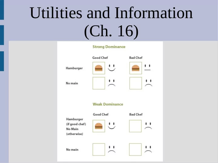
Multivariate Utility Let’s go down to 2 variables (seat, depth): U(seat=left, depth=5m) = 8 U(seat=left, depth=10m) = 5 U(seat=middle, depth=5m) = 6 U(seat=middle, depth=10m) = 7 U(seat=right, depth=5m) = 2 U(seat=right, depth=10m) = 6 “seat=right” is worse for all depth values than “seat=middle”, called strictly dominated

Multivariate Utility What does being strictly dominated tell us? How important are the utilities? (What other assumptions could you make?)

Multivariate Utility If something is strictly dominated, we can ignore the choice in our decision making (as it is always terrible) You can find dominance even if you don’t know the actual utility values, as you quite often know if a factor is “good” or “bad” Let’s change examples from fishing to jobs with properties (fun, pay)

Multivariate Utility Obviously you want a job that pays well and is also exciting, but your job choices are limited to a few options (i.e. actions) McDonalds = (fun=-3, pay=1) Teacher = (fun=4, pay=3) Banker = (fun=0, pay=6) Volunteer = (fun=7, pay=0)

Multivariate Utility You could then plot the possible jobs: Although you do not have a pay-axis utility for jobs Fun and pay are monotonically increasing fun-axis (i.e. more is better)

Multivariate Utility So you can figure dominance as anything that has both better Jobs in this area strictly (or equal) dominate pay and fun pay-axis McDonalds Thus there is no reason to consider McDonalds fun-axis (related to Pareto frontier)

Stochastic Utility However, not all parts might be fixed (i.e. uncertainty) For example, you might want to compute the pay over a couple years, but you don’t know when/if you will get promoted Sometimes you might be stuck doing a boring job (flipping the burgers?) or less boring parts (taking orders?)

Stochastic Utility Thus we could have a range of values (with a distribution) We can still pay-axis have strict dominance if all of one area is up&right of another option fun-axis (i.e. banking)

Stochastic Utility Is there any other way we could define “dominance” when we have probabilities pay-axis and/or distributions? fun-axis

Stochastic Utility You can still have dominance even if you do overlap though, but you need one option to always be better still Consider just the pay side and assume both McDonalds and Teaching is uniformly distributed between [0.5 and 2] and [1.5 and 5] We would call this stochastically dominant

Stochastic Utility Specifically, we need more area under the “worse” curve at all times to be stochastically dominant (from left to right, so more small): distributions for these These integrals can be visualized as (Mc > Teach):

Stochastic Utility Note, this is different than comparing just the expected utility or if you knew the value In these cases you would actually need to know the value of money to figure out if: p*U($0.5) + (1-p)*U($2) > U($1.7) You can use dominance (either type) to eliminate “bad” options, but rarely does this leave you with only 1 choice (so more work)

Utility Simplifications Fortunately, we can avoid specifying an exponential number of utilities (sometimes) We define preference independence as (assuming 3 variables/attributes): Variables x and y and preferentially ind. if (x 1 ,y 1 ) preferred over (x 2 ,y 1 ) means for all y: (x 1 ,y) preferred over (x 2 ,y)

Utility Simplifications This may seem like a strong requirement, but it is normally true (if the things you are measuring (i.e. axis) are independent) For example: Job1=(fun=2, pay=3), Job2=(fun=1, pay=3) ... You prefer Job1 over Job2 (more fun) But this is true for any pay amount: (A›B) JobA=(fun=2, pay=x), JobB=(fun=1, pay=x)

Utility Simplifications We can expand this definition to sets of variables as well: JobA=(fun=2,dist=3,pay=5,time=8) JobB=(fun=4,dist=1,pay=5,time=8) JobA prefered to JobB (more fun, closer) We would say the set {fun,dist} is preferentially independent of {pay,time} if: (fun=2,dist=3,pay=x,time=y) preferred to (fun=4,dist=1,pay=x,time=y) for any x,y

Utility Simplifications If in a subset of variables, A, all are preference independent from each other (over all subsets of A), then mutually preference independent Then, you can actually say their utility is additive! (very non-exponential work) U(fun=w,pay=x,dist=y,time=z) = a*U(fun=w) + b*U(pay=x) + c*U(dist=y) +d*U(time=z)

Utility Simplifications So far we have been assuming the variables have “fixed” values (i.e. no uncertainty) Things become a bit more problematic if we involve probabilities... We can still have “mutual independence”, though this time we call it mutually utility independent (not mutual preference ind.)

Utility Simplifications Thankfully, utility independence is similar to preference independence A random variable x is independent to a (random or normal) variable y if: (x 1 ,y 1 ) preferred over (x 2 ,y 1 ) means for all y: (x 1 ,y) preferred over (x 2 ,y)

Utility Simplifications Going back to the job example, say you have a random variables x 1 , x 2 : x 1 = [(0.5, $2), (0.5, $4)] x 2 = [(0.2, $0), (0.8, $6)] Assume you prefer JobA over JobB in: JobA(fun=2, pay=x 1 ), JobB(fun=2, pay=x 2 ) If utility independent, true for any “fun” z: JobA(fun=z, pay=x 1 ) › JobB(fun=z, pay=x 2 )

Utility Simplifications Unfortunately in the probability case, this independence does not lead to simple additive Instead, utility independence for set {a,b,c}: Or in general: different utility functions as one is for “fun” and another for “pay” why it’s also called “multiplicative” independence

Utility Simplifications You can get an additive utility function even with random variables, but you need another fact to hold true: We need to be able to treat the combination of variables as random variables as well, like: OptionA = [(0.5, x 1 ), (0.5, y 1 )] OptionB = [(0.5, y 1 ), (0.5, y 2 )]

Utility Simplifications Going back to the job example, assume 2 “pay” variables (x 1 , x 2 ) and 2 “fun” (y 1 , y 2 ) If we work at McDonalds, 50% which position [(0.5, (pay=x 1 ,fun=y 1 )), (0.5, (pay=x 2 ,fun=y 2 ))] Suppose another job somewhere else has: [(0.5, (pay=x 1 ,fun=y 2 )), (0.5, (pay=x 2 ,fun=y 1 ))] swap If these jobs are “equal”, then also additive

Utility Simplifications There are some more nitty-gritty cases, like when x is utility independent of y... but you could have y not be independent of x You could see this in a pay “by the hour” job “pay” would be independent of “time” (more pay always better with same time on job)... ...but “time” not independent with “pay” (might want to take more/less time on job)

Utility Simplifications Giving actual numbers to this: Assume you want to make over $20,000 a year (above poverty line... for a family of 3) So you are very unhappy (utility) if you get below this amount, but over this amount your happiness only increases slowly Job1=($15k, 40 hr/w), Job2=($15k, 80 hr/w) Job3=($25k, 40 hr/w), Job4=($25k, 80 hr/w)

Utility Simplifications Job1=($15k, 40 hr/w), Job2=($15k, 80 hr/w) Job3=($25k, 40 hr/w), Job4=($25k, 80 hr/w) Up and down, more pay is always better But if you didn’t have Job3 as an option, the best might be Job4 (sell your soul...) This means you would prefer Job4 over Job1, which has a higher $/hr pay (or not work 80hr)

Utility Simplifications Job1=($15k, 40 hr/w), Job2=($15k, 80 hr/w) Job3=($25k, 40 hr/w), Job4=($25k, 80 hr/w) Up and down, more pay is always better But if you didn’t have Job3 as an option, the best might be Job4 (sell your soul...) This means you would prefer Job4 over Job1, which has a higher $/hr pay (or not work 80hr)

Utility of Information Now that we can compute values (in a hopefully non-exponential way) we can also measure how “useful” information is Remember from last time expected utility is: alpha is argmax a (the a which is the best) probability taking action a makes you end up in state s’ when you know e We can now see the benefit of different information (via utility)