Universal hashing Problem: if h is fixed there are - - PowerPoint PPT Presentation

Universal hashing

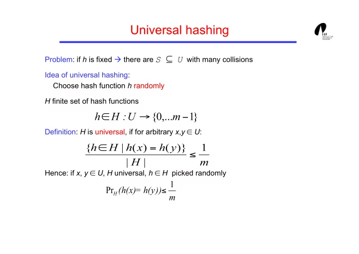
Problem: if h is fixed  there are with many collisions Idea of universal hashing: Choose hash function h randomly H finite set of hash functions Definition: H is universal, if for arbitrary x,y ∈ U: Hence: if x, y ∈ U, H universal, h ∈ H picked randomly

A universal class of hash functions

Assumptions:

• |U| < p (p prime) and U = {0, …, p-1}
• Let a ∈ {1, …, p-1}, b ∈ {0, …, p-1} and ha,b : U  {0,…,m-1} be defined as follows

ha,b = ((ax+b) mod p) mod m Then: The set H = {ha,b | 1 ≤ a ≤ p-1, 0 ≤ b ≤ p-1} is a universal class of hash functions.

Universal hashing - example

Hash table T of size 3, |U| = 5 Consider the 20 functions (set H ): x+0

2x+0 3x+0 4x+0 x+1 2x+1 3x+1 4x+1 x+2 2x+2 3x+2 4x+2 x+3 2x+3 3x+3 4x+3 x+4 2x+4 3x+4 4x+4

each (mod 5) (mod 3)‏ and the key s 1 und 4, let us consider the number of hash functions in H, such that h(1) = h(4). 1 2 3 4 2 3 4 5 3 4 5 6 4 5 6 7 5 6 7 8 1 2 3 4 2 3 4 0 3 4 0 1 4 0 1 2 0 1 2 3 a(1) +b h’(1)=(a(1) +b) mod 5 4 8 12 16 5 9 13 17 6 10 14 18 7 11 15 19 8 12 16 20 a(4) +b 4 3 2 1 0 4 3 2 1 0 4 3 2 1 0 4 3 2 1 0 h’(4)=(a(4) +b) mod 5

Universal hashing - example

Hash table T of size 3, |U| = 5 Consider the 20 functions (set H ): x+0

2x+0 3x+0 4x+0 x+1 2x+1 3x+1 4x+1 x+2 2x+2 3x+2 4x+2 x+3 2x+3 3x+3 4x+3 x+4 2x+4 3x+4 4x+4

each (mod 5) (mod 3)‏ and the keys 1 und 4, let us consider the number of hash functions h in H, such that h(1) = h(4). 1 2 3 4 2 3 4 5 3 4 5 6 4 5 6 7 5 6 7 8 1 2 3 4 2 3 4 0 3 4 0 1 4 0 1 2 0 1 2 3 a(1) +b h’(1)=(a(1) +b) mod 5 4 8 12 16 5 9 13 17 6 10 14 18 7 11 15 19 8 12 16 20 a(4) +b 4 3 2 1 0 4 3 2 1 0 4 3 2 1 0 4 3 2 1 0 h’(4)=(a(4) +b) mod 5

A universal class of hash functions

Assumptions:

• |U| < p (p prime) and U = {0, …, p-1}
• Let a ∈ {1, …, p-1}, b ∈ {0, …, p-1} and ha,b : U  {0,…,m-1} be defined as follows

ha,b = ((ax+b) mod p) mod m Then: The set H = {ha,b | 1 ≤ a ≤ p-1, 0 ≤ b ≤ p-1} is a universal class of hash functions.

ha,b = ((ax+b) mod p) mod m

H = {ha,b | 1 ≤ a ≤ p-1, 0 ≤ b ≤ p-1} is a universal class of hash functions. Proof Consider two distinct keys x and y from {0,…,p-1}, so that x ≠ y. For a given hash function ha,b , we let s = (ax + b) mod p, t = (ay + b) mod p. Firstly, s ≠ t holds, since s - t ≡ a(x - y) (mod p).

Possible ways of treating collisions

Treatment of collisions:

• Collisions are treated differently in different methods.
• A data set with key s is called a colliding element if bucket Bh(s) is already taken by

another data set.

• What can we do with colliding elements?
• 1. Chaining: Implement the buckets as linked lists. Colliding elements are stored in

these lists.

• 2. Open Addressing: Colliding elements are stored in other vacant buckets. During

storage and lookup, these are found through so-called probing.

Theory I Algorithm Design and Analysis

(6 Hashing: Chaining)

• Prof. Th. Ottmann

Chaining (1)

• The hash table is an array (length m) of lists.

Each bucket is realized by a list. class hashTable {

List[] ht; // an array of lists hashTable (int m){ // Construktor ht = new List[m]; for (int i = 0; i < m; i++) ht[i] = new List(); // Construct a list } ... }

• Two different ways of using lists:
• 1. Direct chaining:

Hash table only contains list headers; the data sets are stored in the lists.

• 2. Separate chaining:

Hash table contains at most one data set in each bucket as well as a list header. Colliding elements are stored in the list.

Hashing by chaining

Keys are stored in overflow lists This type of chaining is also known as direct chaining. h(k) = k mod 7 0 1 2 3 4 5 6 hash table T pointer colliding elements 15 2 43 53 12 19 5

Chaining

Lookup key k

• Compute h(k) and overflow list T[h(k)]
• Look for k in the overflow list

Insert a key k

• Lookup k (fails)
• Insert k in the overflow list

Delete a key k

• Lookup k (successfully)
• Remove k from the overflow list

 only list operations

Analysis of direct chaining

Uniform hashing assumption:

• All hash addresses are chosen with the same probability, i.e.:

Pr(h(ki) = j) = 1/m

• independent from operation to operation

Average chain length for n entries: n/m = Definition: C´n = Expected number of entries inspected during a failed search Cn = Expected number of entries inspected during a successful search Analysis:

C'n = α Cn ≈1+ α 2

Chaining

Advantages: + Cn and C´n are small + > 1 possible + real distances + suitable for secondary memory Efficiency of lookup

Cn (successful) C´n (fail) 0.50 1.250 0.50 0.90 1.450 0.90 0.95 1.457 0.95 1.00 1.500 1.00 2.00 2.000 2.00 3.00 2.500 3.00

Disadvantages:

• Additional space for pointers
• Colliding elements are outside the hash table

Summary

Analysis of hashing with chaining:

• worst case:

h(s) always yields the same value, all data sets are in a list. Behavior as in linear lists.

• average case:

– Successful lookup & delete: complexity (in inspections) ≈ 1 + 0.5 × load factor – Failed lookup & insert: complexity ≈ load factor This holds for direct chaining, with separate chaining the complexity is a bit higher.

• best case:

lookup is an immediate success: complexity ∈ O(1).