SLIDE 1 Unit 4: Inference for numerical data
STA 104 - Summer 2017
Duke University, Department of Statistical Science
Slides posted at http://www2.stat.duke.edu/courses/Summer17/sta104.001-1/
Announcements ▶ Project proposal has been uploaded to course webpage
– Read the project instructions carefully – Start discussing with your group about the research questions – Start working on the proposal before your lab on Monday June 12
▶ PS4 and PA4 due Friday! ▶ RA5 on Friday: I’m traveling
1
Reminder: Not every statistically significant result is practically significant ▶ Real differences between the point estimate and null value are
easier to detect with larger samples
▶ However, very large samples will result in statistical significance
even for tiny differences between the sample mean and the null value (effect size), even when the difference is not practically significant
▶ This is especially important to research: if we conduct a study,
we want to focus on finding meaningful results (we want
- bserved differences to be real but also large enough to matter).
▶ The role of a statistician is not just in the analysis of data but
also in planning and design of a study.
“To call in the statistician after the experiment is done may be no more than asking him to perform a post-mortem examination: he may be able to say what the experiment died of.” – R.A. Fisher
2
Reminder: Hypothesis tests have error rates associated with them
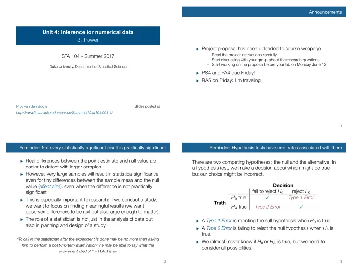
There are two competing hypotheses: the null and the alternative. In a hypothesis test, we make a decision about which might be true, but our choice might be incorrect. Decision fail to reject H0 reject H0 H0 true ✓ Type 1 Error Truth HA true Type 2 Error ✓
▶ A Type 1 Error is rejecting the null hypothesis when H0 is true. ▶ A Type 2 Error is failing to reject the null hypothesis when HA is
true.
▶ We (almost) never know if H0 or HA is true, but we need to
consider all possibilities.
3
SLIDE 2
Reminder: Type 1 error rate = significance level ▶ As a general rule we reject H0 when the p-value is less than
0.05, i.e. we use a significance level of 0.05, α = 0.05.
▶ This means that, for those cases where H0 is actually true, we
will incorrectly reject it at most 5% of the time.
▶ In other words, when using a 5% significance level there is
about 5% chance of making a Type 1 error. P(Type 1 error) = P(Reject H0|H0 is true) = α
▶ This is why we prefer small values of α – increasing α increases
the Type 1 error rate.
4
Filling in the table...
Decision fail to reject H0 reject H0 H0 true 1 − α Type 1 Error, α Truth HA true Type 2 Error, β Power, 1 − β
▶ Type 1 error is rejecting H0 when you shouldn’t have, and the
probability of doing so is α (significance level)
▶ Type 2 error is failing to reject H0 when you should have, and
the probability of doing so is β (a little more complicated to calculate)
▶ Power of a test is the probability of correctly rejecting H0, and
the probability of doing so is 1 − β
▶ In hypothesis testing, we want to keep α and β low, but there
are inherent trade-offs.
5
Type 2 error rate
If the alternative hypothesis is actually true, what is the chance that we make a Type 2 Error, i.e. we fail to reject the null hypothesis even when we should reject it?
▶ The answer is not obvious, but
– If the true population average is very close to the null hypothesis value, it will be difficult to detect a difference (and reject H0). – If the true population average is very different from the null hypothesis value, it will be easier to detect a difference.
▶ Therefore, β must depend on the effect size (δ) in some way
To increase power / decrease β: increase n, increase δ, or increase α
6
Example - Medical history surveys
A medical research group is recruiting people to complete short surveys about their medical history. For example, one survey asks for information on a person’s family history in regards to cancer. Another survey asks about what topics were discussed during the person’s last visit to a hospital. So far, on average people complete an average of 4 surveys, with the standard deviation of 2.2 surveys. The research group wants to try a new interface that they think will encourage new enrollees to complete more surveys, where they will randomize a total of 300 enrollees to either get the new interface or the current interface (equally distributed between the two groups). What is the power of the test that can detect an increase of 0.5 surveys per enrollee for the new interface compared to the old interface? Assume that the new interface does not affect the standard deviation of completed surveys, and α = 0.05.
7
SLIDE 3 Calculating power
The preceeding question can be rephrased as – How likely is it that we can reject a null hypothesis of H0 : µnew − µcurrent = 0 if the new interface results in an increase of 0.5 surveys per enrollee, on average? Let’s break this down into two simpler problems:
- 1. Problem 1: Which values of (¯
xnew − ¯ xcurrent) represent sufficient evidence to reject this H0?
- 2. Problem 2: What is the probability that we would reject this H0
if ¯ xnew − ¯ xcurrent had come from a distribution with µnew − µcurrent = 0.5, i.e. what is the probability that we can
- btain such an observed difference from this distribution?
8
Problem 1
Which values of (¯ xnew interface − ¯ xold interface) represent sufficient evidence to reject H0? H0 : µnew − µcurrent = 0 HA : µnew − µcurrent > 0 nnew = ncurrent = 150
9
Problem 1 - cont.
Clicker question
What is the lowest t-score that will allow us to reject the null hypothesis in favor of the alternative? H0 : µnew − µcurrent = 0 HA : µnew − µcurrent > 0 nnew = ncurrent = 150, α = 0.05 (a) 1.65 (b) 1.66 (c) 1.96 (d) 1.98 (e) 2.63
t* = ?
0.05 10
Problem 1 - cont.
Clicker question
Which values of (¯ xnew − ¯ xcurrent) represent sufficient evidence to reject H0? H0 : µnew − µcurrent = 0 HA : µnew − µcurrent > 0 nnew = ncurrent = 150, α = 0.05, snew = 2.2 = scurrent = 2.2
(a) ¯ xnew − ¯ xcurrent < −0.42 (b) ¯ xnew − ¯ xcurrent > −0.42 (c) ¯ xnew − ¯ xcurrent < 0.42 (d) ¯ xnew − ¯ xcurrent > 0.42 (e) ¯ xnew − ¯ xcurrent > 1.66
11
SLIDE 4 Problem 2
Clicker question
What is the probability that we would reject this H0 if ¯ xnew − ¯ xcurrent had come from a distribution with µnew − µcurrent = 0.5, i.e. what is the probability that we can obtain such an observed difference from this distribution? H0 : µnew − µcurrent = 0 HA : µnew − µcurrent > 0 nnew = ncurrent = 150, α = 0.05, snew = 2.2 = scurrent = 2.2
(a) 5% (b) 38% (c) 62% (d) 80% (e) 95%
12
Problem 2 - cont.
Clicker question
What is β, the Type 2 error rate? (a) 5% (b) 38% (c) 62% (d) 80% (e) 95%
13
Achieving desired power
There are several ways to increase power (and hence decrease Type 2 error rate):
- 1. Increase the sample size.
- 2. Decrease the standard deviation of the sample, which is
equivalent to increasing the sample size (it will decrease the standard error). With a smaller s we have a better chance of distinguishing the null value from the observed point estimate. This is difficult to ensure but cautious measurement process and limiting the population so that it is more homogenous may help.
- 3. Increase α, which will make it more likely to reject H0 (but note
that this has the side effect of increasing the Type 1 error rate).
- 4. Consider a larger effect size. If the true mean of the population
is in the alternative hypothesis but close to the null value, it will be harder to detect a difference.
14
Recap - Calculating Power ▶ Step 0: Pick a meaningful effect size δ and a significance level α ▶ Step 1: Calculate the range of values for the point estimate
beyond which you would reject H0 at the chosen α level.
▶ Step 2: Calculate the probability of observing a value from
preceding step if the sample was derived from a population where µ = µH0 + δ
15
SLIDE 5 Back to medical surveys... How large a sample size would you need if you wanted 90% power to detect a 0.5 increase in average number of surveys taken at the 5% significance level? H0 : µnew − µcurrent = 0, HA : µnew − µcurrent > 0 nnew = ncurrent =?, snew = 2.2 = scurrent = 2.2 δ = 0.5, α = 0.05, power = 90%, β = 0.10
200 400 600 800 1000 0.2 0.4 0.6 0.8 1.0 power
When n > 334, power is at least 90%.
16
If you're interested...
s = 2.2 mu = 0 delta = 0.5 ns = 10:1000 power = rep(NA, length(ns)) for(i in 10:1000){ n = i t_star = qt(0.95, df = n-1) se = sqrt((s^2 / n) + (s^2 / n)) cutoff = t_star * se t_cutoff = (cutoff - (mu+delta)) / se power[i-9] = pt(t_cutoff, df = n-1, lower.tail = FALSE) } which_n = which.min(abs(power - 0.9)) power[which_n] power[which_n + 1] ns[which_n + 1] 17
Application exercise: 4.3
See course website for details.
18
Summary of main ideas
- 1. Not every statistically significant result is practically significant
- 2. Hypothesis tests have error rates associated with them
- 3. Type 1 error rate = significance level
- 4. Calculating the power is a two step process
- 5. Power goes up with effect size and sample size, and is
inversely proportional with significance level and standard error
- 6. A priori power calculations determine desired sample size
19