Understanding complex information-processing systems Marr (1982) - - PowerPoint PPT Presentation

Understanding complex information-processing systems

Marr (1982)

Computational theory What is the goal of the computation, why is it appropriate, and what is the logic of the strategy by which it can be carried out? Representation and algorithm How can this computational theory be implemented? What is the representation for the input and output, and what is the algorithm for the transformation? Hardware implementation How can the representation and algorithm be realized physically?

1 / 1 2 / 1 3 / 1

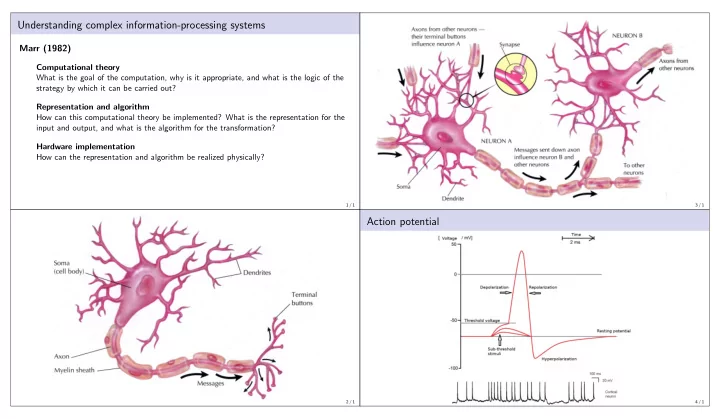
Action potential

4 / 1

5 / 1

Notation

i, j indices of units (i sending, j receiving) aj activation of unit j nj summed net input to unit j wij weight on connection from unit i to unit j ej external input to unit j θj threshold for unit j bj bias (tonic input) to unit j (= −θj)

6 / 1

Types of units

Binary threshold unit nj =

• i

aiwij + ej aj = 1 if nj > θj

• therwise

If “bias” bj = −θj, this is the same as nj =

• i

aiwij + ej + bj aj = 1 if nj > 0

• therwise

Will generally omit bj and ej in equations Bias bj can be treated as weight wij from special unit with fixed activation ai = 1. External input ej can be treated as incoming activation ai across connection with fixed weight wij = 1.

7 / 1

Linear units aj = nj =

• i

aiwij Rectified linear units (ReLUs) aj = max (0.0, nj) Sigmoidal (“logistic”, “semi-linear”) units aj = σ(nj) = 1 1 + exp (−nj) Binary stochastic units p (aj = 1) = 1 1 + exp (−nj)

8 / 1

Continuous time-averaged (cascaded) units [two alternatives] n[t]

j

= τ

• i

a[t−1]

i

wij + (1 − τ) n[t−1]

j

a[t]

j

= τ σ

• n[t]

j

• +

(1 − τ) a[t−1]

j

Interactive activation (Jets & Sharks model; Schema model; McClelland & Rumelhart letter/word model) n[t]

j

=

• i

a[t−1]

i

wij + e[t]

j

a[t]

j

= (1 − decay) a[t−1]

j

+    n[t]

j

• max − a[t−1]

j

• if n[t]

j

> 0 n[t]

j

• a[t−1]

j

− min

• therwise

decay = 0.1 max = 1.0 min = −0.2

9 / 1