uncertainty rn2 sec 13 1 13 6 rn3 sec 13 1 13 5
play

Uncertainty [RN2 Sec. 13.1-13.6] [RN3 Sec. 13.1-13.5] CS 486/686 - PDF document

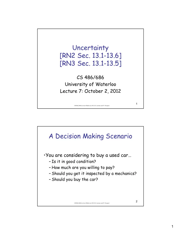
Uncertainty [RN2 Sec. 13.1-13.6] [RN3 Sec. 13.1-13.5] CS 486/686 University of Waterloo Lecture 7: October 2, 2012 1 CS486/686 Lecture Slides (c) 2012 K. Larson and P. Poupart A Decision Making Scenario You are considering to buy a used


  1. Uncertainty [RN2 Sec. 13.1-13.6] [RN3 Sec. 13.1-13.5] CS 486/686 University of Waterloo Lecture 7: October 2, 2012 1 CS486/686 Lecture Slides (c) 2012 K. Larson and P. Poupart A Decision Making Scenario •You are considering to buy a used car… – Is it in good condition? – How much are you willing to pay? – Should you get it inspected by a mechanics? – Should you buy the car? 2 CS486/686 Lecture Slides (c) 2012 K. Larson and P. Poupart 1

  2. In the next few lectures • Probability theory – Model uncertainty • Utility theory – Model preferences • Decision theory – Combine probability theory and utility theory 3 CS486/686 Lecture Slides (c) 2012 K. Larson and P. Poupart Introduction • Logical reasoning breaks down when dealing with uncertainty • Example: Diagnosis –  p Symptom(p,Toothache)  Disease(p, Cavity) • But not all people with toothaches have cavities… –  p Symptom(p, Toothache)  Disease(p,Cavity) v Disease(p,Gumdisease) v Disease(p, Hit in the Jaw) v … • Can’t enumerate all possible causes and not very informative –  p Disease(p, Cavity)  Symptom(p,Toothache) • Does not work since not all cavities cause toothaches… 4 CS486/686 Lecture Slides (c) 2012 K. Larson and P. Poupart 2

  3. Introduction • Logic fails because – We are lazy • Too much work to write down all antecedents and consequences – Theoretical ignorance • Sometimes there is just no complete theory – Practical ignorance • Even if we knew all the rules, we might be uncertain about a particular instance (not collected enough information yet) 5 CS486/686 Lecture Slides (c) 2012 K. Larson and P. Poupart Probabilities to the rescue • For many years AI danced around the fact that the world is an uncertain place • Then a few AI researchers decided to go back to the 18 th century – Revolutionary – Probabilities allow us to deal with uncertainty that comes from our laziness and ignorance – Clear semantics – Provide principled answers for • Combining evidence, predictive and diagnostic reasoning, incorporation of new evidence – Can be learned from data – Intuitive for humans (?) 6 CS486/686 Lecture Slides (c) 2012 K. Larson and P. Poupart 3

  4. Discrete Random Variables • Random variable A describes an outcome that cannot be determined in advance (i.e. roll of a dice) – Discrete random variable means that its possible values come from a countable domain (sample space) • E.G If X is the outcome of a dice throw, then X  {1,2,3,4,5,6} – Boolean random variable A  {True, False} • A = The Canadian PM in 2040 will be female • A = You have Ebola • A = You wake up tomorrow with a headache 7 CS486/686 Lecture Slides (c) 2012 K. Larson and P. Poupart Events • An event is a complete specification of the state of the world in which the agent is uncertain – Subset of the sample space • Example: – Cavity=True Λ Toothache=True – Dice=2 • Events must be – Mutually exclusive – Exhaustive (at least one event must be true) 8 CS486/686 Lecture Slides (c) 2012 K. Larson and P. Poupart 4

  5. Probabilities • We let P(A) denote the “degree of belief” we have that statement A is true – Also “fraction of worlds in which A is true” • Philosophers like to discuss this (but we won’t) • Note: – P(A) DOES NOT correspond to a degree of truth – Example: Draw a card from a shuffled deck • The card is of some type (e.g ace of spades) • Before looking at it P(ace of spades) = 1/52 • After looking at it P(ace of spades) = 1 or 0 9 CS486/686 Lecture Slides (c) 2012 K. Larson and P. Poupart Visualizing A Event space of all possible worlds. Worlds in which A is true It’s area is 1 Worlds in which A is False P(A) = Area of oval 10 CS486/686 Lecture Slides (c) 2012 K. Larson and P. Poupart 5

  6. The Axioms of Probability • 0  P(A)  1 • P(True) = 1 • P(False) = 0 • P(A v B) = P(A) + P(B) - P(A Λ B) • These axioms limit the class of functions that can be considered as probability functions 11 CS486/686 Lecture Slides (c) 2012 K. Larson and P. Poupart Interpreting the axioms • 0  P(A)  1 • P(True) = 1 • P(False) = 0 • P(A v B) = P(A) + P(B) - P(A Λ B) The area A zero area of A would mean can’t be no world smaller could ever than 0 have A as true 12 CS486/686 Lecture Slides (c) 2012 K. Larson and P. Poupart 6

  7. Interpreting the axioms • 0  P(A)  1 • P(True) = 1 • P(False) = 0 • P(A v B) = P(A) + P(B) - P(A Λ B) The area An area of of A 1 would can’t be mean all larger possible than 1 worlds have A as true 13 CS486/686 Lecture Slides (c) 2012 K. Larson and P. Poupart Interpreting the axioms • 0  P(A)  1 • P(True) = 1 • P(False) = 0 • P(A v B) = P(A) + P(B) - P(A Λ B) A Λ B A B 14 CS486/686 Lecture Slides (c) 2012 K. Larson and P. Poupart 7

  8. Take the axioms seriously! • There have been attempts to use different methodologies for uncertainty – Fuzzy logic, three valued logic, Dempster- Shafer, non-monotonic reasoning,… • But if you follow the axioms of probability then no one can take advantage of you  15 CS486/686 Lecture Slides (c) 2012 K. Larson and P. Poupart A Betting Game [di Finetti 1931] • Propositions A and B • Agent 1 announces its “degree of belief” in A and B (P(A) and P(B)) • Agent 2 chooses to bet for or against A and B at stakes that are consistent with P(A) and P(B) • If Agent 1 does not follow the axioms, it is guaranteed to lose money Agent 1 Agent 2 Outcome for Agent 1 Proposition Belief Bet Odds A Λ B A Λ ~B ~A Λ B ~A Λ ~B A 0.4 A 4 to 6 -6 -6 4 4 B 0.3 B 3 to 7 -7 3 -7 3 AVB 0.8 ~(AVB) 2 to 8 2 2 2 -8 -11 -1 -1 -1 16 CS486/686 Lecture Slides (c) 2012 K. Larson and P. Poupart 8

  9. Theorems from the axioms • Thm: P(~A)=1-P(A) • Proof: P(AV~A)=P(A)+P(~A)-P(A Λ ~A) P(True)=P(A)+P(~A)-P(False) 1 = P(A)+P(~A)-0 P(~A)=1-P(A) 17 CS486/686 Lecture Slides (c) 2012 K. Larson and P. Poupart Theorems from axioms • Thm: P(A) = P(A Λ B) + P(A Λ ~B) • Proof: For you to do Why? Because it is good for you 18 CS486/686 Lecture Slides (c) 2012 K. Larson and P. Poupart 9

  10. Multivalued Random Variables • Assume domain of A (sample space) is {v 1 , v 2 , …, v k } • A can take on exactly one value out of this set – P(A=v i Λ A=v j ) = 0 if i  j – P(A=v 1 V A=v 2 V … V A=v k ) = 1 19 CS486/686 Lecture Slides (c) 2012 K. Larson and P. Poupart Terminology • Probability distribution: – A specification of a probability for each event in our sample space – Probabilities must sum to 1 • Assume the world is described by two (or more) random variables – Joint probability distribution • Specification of probabilities for all combinations of events 20 CS486/686 Lecture Slides (c) 2012 K. Larson and P. Poupart 10

  11. Joint distribution • Given two random variables A and B: • Joint distribution: – Pr(A=a Λ B=b) for all a,b • Marginalisation (sumout rule): – Pr(A=a) = Σ b Pr(A=a Λ B=b) – Pr(B=b) = Σ a Pr(A=a Λ B=b) 21 CS486/686 Lecture Slides (c) 2012 K. Larson and P. Poupart Example: Joint Distribution sunny ~sunny cold ~cold cold ~cold headache 0.072 0.008 headache 0.108 0.012 ~headache 0.144 0.576 ~headache 0.016 0.064 P(headache Λ sunny Λ cold) = 0.108 P(~headache Λ sunny Λ ~cold) = 0.064 P(headacheVsunny) = 0.108 + 0.012 + 0.072 + 0.008 + 0.016 + 0.064 = 0.28 P(headache) = 0.108 + 0.012 + 0.072 + 0.008 = 0.2 marginalization 22 CS486/686 Lecture Slides (c) 2012 K. Larson and P. Poupart 11

  12. Conditional Probability • P(A|B) fraction of worlds in which B is true that also have A true H=“Have headache” F=“Have Flu” F P(H)=1/10 P(F)=1/40 P(H|F)=1/2 H Headaches are rare and flu is rarer, but if you have the flu, then there is a 50-50 chance you will have a headache 23 CS486/686 Lecture Slides (c) 2012 K. Larson and P. Poupart Conditional Probability F P(H|F)= Fraction of flu inflicted worlds in which you have a headache H =(# worlds with flu and headache)/ (# worlds with flu) = (Area of “H and F” region)/ H=“Have headache” (Area of “F” region) F=“Have Flu” = P(H Λ F)/ P(F) P(H)=1/10 P(F)=1/40 P(H|F)=1/2 24 CS486/686 Lecture Slides (c) 2012 K. Larson and P. Poupart 12

  13. Conditional Probability • Definition: – P(A|B) = P(A Λ B) / P(B) • Chain rule: – P(A Λ B) = P(A|B) P(B) Memorize these! 25 CS486/686 Lecture Slides (c) 2012 K. Larson and P. Poupart Inference F One day you wake up with a headache. You think “Drat! 50% of flues are associated with headaches so I must have a 50- H 50 chance of coming down with the flu” H=“Have headache” F=“Have Flu” Is your reasoning P(H)=1/10 correct? P(F)=1/40 P(H|F)=1/2 26 CS486/686 Lecture Slides (c) 2012 K. Larson and P. Poupart 13

Download Presentation
Download Policy: The content available on the website is offered to you 'AS IS' for your personal information and use only. It cannot be commercialized, licensed, or distributed on other websites without prior consent from the author. To download a presentation, simply click this link. If you encounter any difficulties during the download process, it's possible that the publisher has removed the file from their server.

Recommend


More recommend