SLIDE 1 ECO 305 — FALL 2003 — November 25
UNCERTAINTY — ALTERNATIVE THEORIES Behavior inconsistent with expected utility theory: Some examples
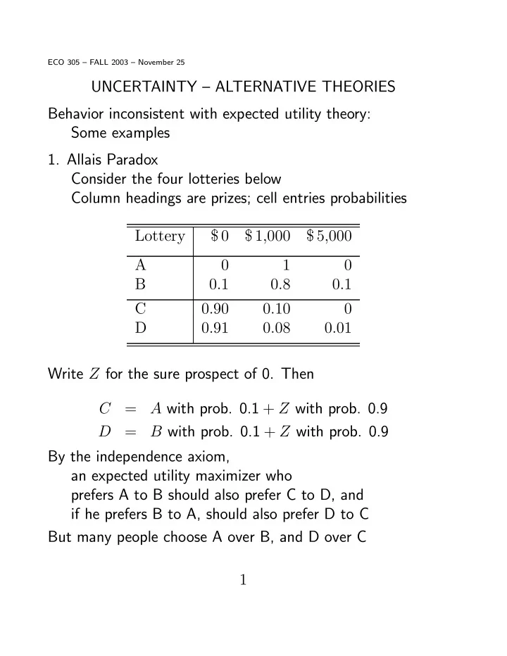
Consider the four lotteries below Column headings are prizes; cell entries probabilities Lottery $ 0 $ 1,000 $ 5,000 A 1 B 0.1 0.8 0.1 C 0.90 0.10 D 0.91 0.08 0.01 Write Z for the sure prospect of 0. Then C = A with prob. 0.1 + Z with prob. 0.9 D = B with prob. 0.1 + Z with prob. 0.9 By the independence axiom, an expected utility maximizer who prefers A to B should also prefer C to D, and if he prefers B to A, should also prefer D to C But many people choose A over B, and D over C 1
SLIDE 2
U(W) W W0
vN-M type utility but with kink at initial wealth Values losses from status quo much more than gains
- 3. Minimizing maximum regret
When comparing choices A and B, regret of A is max
i ∈ Scenarios max( Ui(B) − Ui(A), 0 )
- 4. Errors in calculating probabilities
Treating small probability events as if impossible Not applying correct Bayes’ rule when updating probabilities given some information Expected utility approach still dominates in most applications — finance, game theory etc. But alternatives being explored at research level 2
SLIDE 3 DEMAND FOR INSURANCE Loss L in scenario 2 (prob. π2) Endowments (W0, W0 − L) Each dollar of coverage requires insurance premium p If insurance is actuarially (statistically) fair, p = π2. If buy X dollars of coverage, final wealths W1 = W0 − p X, W2 = W0 − L − p X + X Choose X to maximize EU(W) = π1 U(W0 − p X) + π2 U(W0 − L + (1 − p) X) FONC −p π1 U0(W0−p X)+(1−p) π2 U0(W0−L+(1−p) X) = 0 SOSC is U 00 < 0, risk-aversion. If fair insurance (p = π2, 1 − p = π1) FONC becomes: U 0(W0 − p X) = U 0(W0 − L + (1 − p) X), W1 = W2 so risk is eliminated — full coverage X = L optimum
- Ins. Co.’s expected profit EΠ = p X − π2 X, so
fair insurance will be available if: (1) Risk-neutral insurers (by law of large nos ?) (2) Perfect competition among insurers ⇒ EΠ = 0 (2) No (minimal) admin. costs, no info. asymmetry 3
SLIDE 4
Alternative view: eliminate X from W1, W2 equations: (1 − p) W1 + p W2 = (1 − p) W0 + p (W0 − L) Budget constraint for “contingent claims to dollars” Prices p, (1 − p). Slope = (1 − p)/p Subject to this, max EU = π1 U(W1) + π2 U(W2) Probabilities must be exogenous for symmetric info.
W2 W1 45-deg EU contours (W0 , W0 -L)
If insurance is fair, p = π2 slope of budget line = 45-degree-line-MRS so tangency (optimum) at 45-degree-line If “unfair” (loaded) insurance, p > π2 slope of budget line < 45-degree-line-MRS Less than full insurance is optimal 4
SLIDE 5
TRADING RISK IN MARKETS Markets held before uncertainty is resolved Buy/sell “contingent claims”, like betting slips Simplest of these — Arrow-Debreu Securities (ADS) Basic or elementary scenarios i = 1, 2, . . . n ADSi is claim to $1 if scenario i, nothing otherwise Prices pi paid in advance If money can be stored between now and time when uncertainty resolved and claims settled, P
i pi = 1
If sure int. rate r between now and then, = 1/(1 + r) Equilibrium prices pi depend on probabilities πi and on extent of, and attitudes toward, the risks EXAMPLE 1 — No aggregate risk Individual risk can be fully insured by trade at fair prices Two scenarios Total W same in both Objective Probs. (1/2 each) B more risk-averse than R But MRS on 45-degree π1/π2 = 1 for both So eqm. on that line p1/p2 = π1/π2 5
SLIDE 6
EXAMPLE 2 — Aggregate risk Total W1 > W2: Scenario 1 “good”, 2 “bad” Objective probabilities π1, π2 Pareto efficiency, Core, Equil’m as in GE Theory (Wk.7) ADS’s achive efficient allocation of risk ! B is more risk-averse than R — so efficient points are relatively closer to B’s 45-degree line At any efficient risk-allocation, p1/p2 < π1/π2 Difference depends on risk-aversions of traders If one is risk-neutral, p1/p2 = π1/π2 6