= + U ( s ) R ( s ) max T ( s , a , s ' ) U - - PDF document

SLIDE 1

1

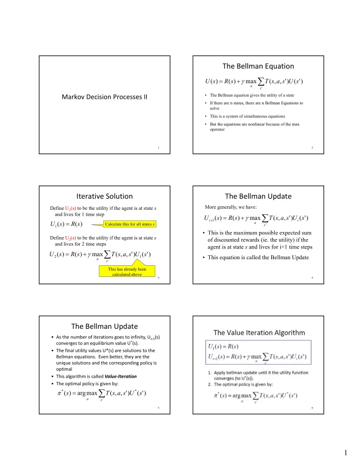
Markov Decision Processes II

1

The Bellman Equation

∑

+ =

'

) ' ( ) ' , , ( max ) ( ) (

s a

s U s a s T s R s U γ

• The Bellman equation gives the utility of a state
• If there are n states, there are n Bellman Equations to

2

, q solve

• This is a system of simultaneous equations
• But the equations are nonlinear because of the max
• perator

Iterative Solution

Define U1(s) to be the utility if the agent is at state s and lives for 1 time step

) ( ) (

1

s R s U =

Calculate this for all states s

3

Define U2(s) to be the utility if the agent is at state s and lives for 2 time steps

∑

+ =

' 1 2

) ' ( ) ' , , ( max ) ( ) (

s a

s U s a s T s R s U γ

This has already been calculated above

The Bellman Update

∑

+ =

+ ' 1

) ' ( ) ' , , ( max ) ( ) (

s i a i

s U s a s T s R s U γ

More generally, we have:

• This is the maximum possible expected sum

4

p p

• f discounted rewards (ie. the utility) if the

agent is at state s and lives for i+1 time steps

• This equation is called the Bellman Update

The Bellman Update

• As the number of iterations goes to infinity, Ui+1(s)

converges to an equilibrium value U*(s).

• The final utility values U*(s) are solutions to the

Bellman equations. Even better, they are the unique solutions and the corresponding policy is

5

q p g p y

• ptimal
• This algorithm is called Value‐Iteration
• The optimal policy is given by:

∑

=

' * *

) ' ( ) ' , , ( max arg ) (

s a

s U s a s T s π

6

SLIDE 2

2

Example

• We will use the following convention when

drawing MDPs graphically:

State Action

7

R(s) Action Transition probability

Example

A +12 A1 B

• 4

B1 0.5 0.5 γ =0.9

8

0.25 0.75 C +2 A2 C1 1.0 0.5 0.5

Example

i=1 U1(A) = R(A)=12 U1(B) = R(B)=‐4 U (C) R(C) 2

9

U1(C) = R(C)=2

Example

i=2 U2(A) = 12 + (0.9) * max{(0.5)(12)+(0.5)(‐4), (1.0)(2)} = 12 + (0 9)*max{4 0 2 0} = 12 + 3 6 = 15 6

U1(A) U1(B) U1(C) 12

• 4

2

10

= 12 + (0.9) max{4.0,2.0} = 12 + 3.6 = 15.6 U2(B) = ‐4 + (0.9) * {(0.25)(12)+(0.75)(‐4)} = ‐4 + (0.9)*0 = ‐4 U2(C) = 2 + (0.9) * {(0.5)(2)+(0.5)(‐4)} = 2 + (0.9)*(‐1) = 2‐0.9 = 1.1

Example

i=3 U3(A) = 12 + (0.9) * max{(0.5)(15.6)+(0.5)(‐ 4) (1 0)(1 1)} = 12 + (0 9) * max{5 8 1 1} = 12 +

U2(A) U2(B) U2(C) 15.6

• 4

1.1

11

4),(1.0)(1.1)} = 12 + (0.9) max{5.8,1.1} = 12 + (0.9)(5.8) = 17.22 U3(B) = ‐4 + (0.9) * {(0.25)(15.6)+(0.75)(‐4)} = ‐4 + (0.9)*(3.9‐3) = ‐4 + (0.9)(0.9) = ‐3.19 U3(C) = 2 + (0.9) * {(0.5)(1.1)+(0.5)(‐4)} = 2 + (0.9)*{0.55‐2.0} = 2 + (0.9)(‐1.45) = 0.695

The Bellman Update

• What exactly is going on?
• Think of each Bellman update as an update
• f each local state
• If we do enough local updates we end up

12

• If we do enough local updates, we end up

propagating information throughout the state space

SLIDE 3

3

Value Iteration on the Maze

13

Notice that rewards are negative until a path to (4,3) is found, resulting in an increase in U

Value‐Iteration Termination

When do you stop? In an iteration over all the states, keep track

• f the maximum change in utility of any state

(call this δ)

14

(call this δ) When δ is less than some pre‐defined threshold, stop This will give us an approximation to the true utilities, we can act greedily based on the approximated state utilities

Comments

Value iteration is designed around the idea of the utilities of the states The computational difficulty comes from the max operation in the bellman equation max operation in the bellman equation Instead of computing the general utility of a state (assuming acting optimally), a much easier quantity to compute is the utility of a state assuming a policy

15 16

γ

Evaluating a Policy

Once we compute the utilities, we can easily improve the current policy by one‐ step look‐ahead: This suggests a different approach for finding optimal policy

17

Policy Iteration

• Start with a randomly chosen initial policy π0
• Iterate until no change in utilities:
• 1. Policy evaluation: given a policy πi, calculate

the utility Ui(s) of every state s using policy πi

18

• 2. Policy improvement: calculate the new policy

πi+1 using one‐step look‐ahead based on Ui(s) ie.

∑

=

+ ' 1

) ' ( ) ' , , ( max arg ) (

s i a i

s U s a s T s π

SLIDE 4

4

Policy Evaluation

• Policy improvement is straightforward
• Policy evaluation requires a simpler

version of the Bellman equation

• Compute U (s) for every state s using π

19

• Compute Ui(s) for every state s using πi:

∑

+ =

'

) ' ( ) ' ), ( , ( ) ( ) (

s i i i

s U s s s T s R s U π γ

Notice that there is no max operator, so the above equations are linear! O(n3) where n is the number of states

Policy Evaluation

• O(n3) is still too expensive for large state spaces
• Instead of calculating exact utilities, we could calculate

approximate utilities

• The simplified Bellman update is:

∑

+ ← ) ' ( ) ' ) ( ( ) ( ) ( s U s s s T s R s U π γ

20

• Repeat the above k times to get the next utility estimate

∑

+ ←

+ ' 1

) ' ( ) ' ), ( , ( ) ( ) (

s i i i

s U s s s T s R s U π γ

This is called modified policy iteration

Comparison

• Which would you prefer, policy or value

iteration?

• Depends…

– If you have lots of actions in each state: policy

21

If you have lots of actions in each state: policy iteration – If you have a pretty good policy to start with: policy iteration – If you have few actions in each state: value iteration

Limitations

• Need to represent the utility (and policy) for

every state

• In real problems, the number of states may be

very large

• Leads to intractably large tables

22

• Leads to intractably large tables
• Need to find compact ways to represent the

states eg

– Function approximation – Hierarchical representations – Memory‐based representations

What you should know

• How value iteration works
• How policy iteration works
• Pros and cons of both

Wh t i th bi bl ith b th l

23

• What is the big problem with both value

and policy iteration