
SLIDE 1
Triangles, Squares and Biautomaticity
Jon McCammond (U.C. Santa Barbara) Rena Levitt (U.C. Santa Barbara)
1
Triangles, Squares and Biautomaticity Jon McCammond (U.C. Santa - - PowerPoint PPT Presentation
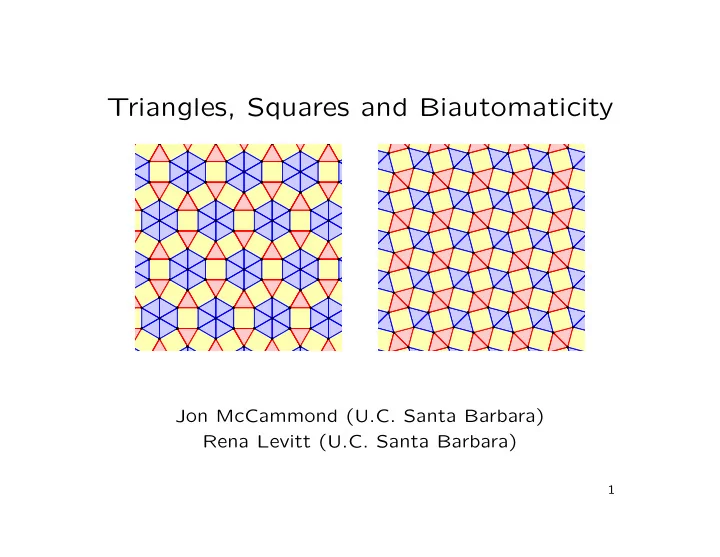
Triangles, Squares and Biautomaticity Jon McCammond (U.C. Santa Barbara) Rena Levitt (U.C. Santa Barbara) 1 The Basic Problems Consider a tiling of the plane by regular triangles and squares. 1) How many such tilings are there? 2) What does a
1
2
3
4
5
NPC △ NPC NPC △ SNPC △n NPC n SNPC △n
6
7
8
9
10
11
12
13
14
15
16
17
18
19
20
21
22
23
24
25
26
27