Topics Background, Definitions, and Prior Theorems Mat 3770 - - PDF document

Mat 3770 Steiner Trees

Spring 2014

1

Topics

◮ Background, Definitions, and Prior Theorems ◮ Initial Algorithms ◮ Theoretical Work ◮ Improved Performance Algorithms ◮ Conclusions

2

Motivation for Studying Steiner Trees

Applications

◮ Communications networks ◮ Mechanical & Electrical systems in buildings and along streets ◮ Wire layout in VLSI chip design

VLSI Chip Design

Given a collection of cells and a collection of nets, find a way to position the cells (placement) and run the wires for net connections (routing) so the wires are short with as few vias as possible, and the whole layout uses a minimum amount of area.

3

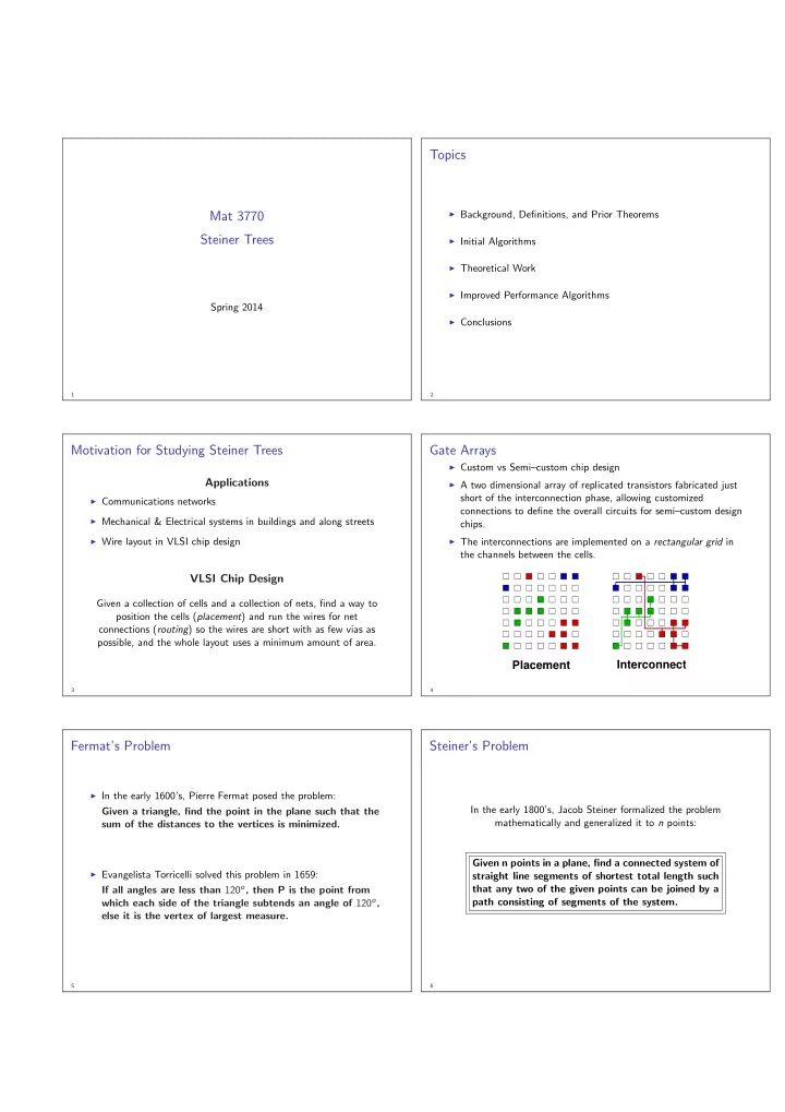
Gate Arrays

◮ Custom vs Semi–custom chip design ◮ A two dimensional array of replicated transistors fabricated just

short of the interconnection phase, allowing customized connections to define the overall circuits for semi–custom design chips.

◮ The interconnections are implemented on a rectangular grid in

the channels between the cells.

Placement Interconnect

4

Fermat’s Problem

◮ In the early 1600’s, Pierre Fermat posed the problem:

Given a triangle, find the point in the plane such that the sum of the distances to the vertices is minimized.

◮ Evangelista Torricelli solved this problem in 1659:

If all angles are less than 120o, then P is the point from which each side of the triangle subtends an angle of 120o, else it is the vertex of largest measure.

5

Steiner’s Problem

In the early 1800’s, Jacob Steiner formalized the problem mathematically and generalized it to n points: Given n points in a plane, find a connected system of straight line segments of shortest total length such that any two of the given points can be joined by a path consisting of segments of the system.

6

Spanning Trees

Related Problem: Minimal Spanning Trees

A C D E F G B

Steiner Minimal Trees: shorten trees by adding points

A D E F G B C

7

Shortest Rectilinear Steiner Spanning Tree Problem

Connecting a set of points in the plane with a connected collection of vertical and horizontal lines with minimal overall length.

Steiner Spanning Tree Shortest Rectilinear

flip connections and take out overlaps

Spanning Tree Rectilinear Minimal

8

Upper and Lower Bounds

• Theorem. (Hwang) An SRSST over a set of points is no smaller

in length than two thirds the length of the RMST over the same set of points. SRSST RMST This gives us nice upper (Length(RMST)) and lower ( 2

3 Length(RMST))

bounds on the length of Steiner trees.

9

Grid & Enclosing Rectangle

◮ Theorem. (Hannan) An SRSST over a set of points exists on

the grid induced by the points.

◮ Note: The shortest path between two points is not unique.

Thus a solution to the SRSST Problem in general is not unique.

◮ The Enclosing Rectangle is the smallest rectangle containing

the point set. Any SRSST must be at least half the perimeter of the enclosing rectangle. (Providing another lower bound.)

10

Grid Segments

j k q a c b e d r h

• v

i p w x l s t m f g n u

Points and Their Induced Grid Number of Segments (Horizontal & Vertical) × n nodes × (n − 1) edges 4 points: 2 × 4 × 3 = 24 grid segments 5 points: 2 × 5 × 4 = 40 grid segments 6 points: 2 × 6 × 5 = 60 grid segments

11

NP–Complete Problem

• Theorem. (Garey and Johnson) The problem of determining the

minimum length of an optimal rectilinear Steiner tree for a set of points in the plane is NP–Complete. This implies it is probable that finding an optimal solution will take worse than polynomial time. That may be alright for small problems, but heuristic algorithms are still needed. Heuristic Algorithms Non–optimal, but usually close & have performance guarantees

12

Research Sequence

◮ Extended Kruskal ◮ Na¨

ıve Branch and Bound (optimal)

◮ Structural Theorems ◮ Pretaxial & Epitaxial Branch and Bound (optimal) ◮ MST–based Direction Assignment ◮ Simulated Annealing ◮ Stochastic Evolution

13

Extended Kruskal

◮ Based on Kruskal’s MST algorithm:

Place all points in individual subtrees Repeat Connect closest subtrees Until a single tree is formed

◮ Two versions with different connection schemes:

All grid intersection Only corner points considered points considered

◮ Theorem. The EK algorithm is correct and produces an RSST

no larger than the RMST. Guarantees result is no worse than 150% of optimal .

14

Na¨ ıve Branch and Bound

Idea: look at all combinations of grid edges. General Branch and Bound Method Examine all feasible solutions in an orderly manner: Organize the search space as a tree Search the tree using a depth first approach Using lower and upper bounds to decrease the search

15

Grid and Search Tree

l k j i h f g c d e b a

Induced Grid over three points

b b c bc a a a ab ab abc ac

. . . etc . . . Na¨ ıve Search Tree

16

Pruning the Search Tree

◮ A small search space is needed to feasibly complete the tree

traversal, so we prune the tree:

◮ lower bound: larger of 2

3 RMST or 1 2 perimeter

◮ upper bound: RMST or result of heuristic

◮ If collection of grid edges is

◮ too large — discard ◮ too short — discard ◮ if they form a tree and it’s shorter than current known tree, keep

it

◮ Unfortunately, there were still too many combinations to check

17

Implementation

◮ All combinations of grid edges considered

Search Space: O(22n(n−1)) 3 points yield 212 or 4096 combinations

◮ Implementation: essentially used a binary odometer where

1 = IN and 0 = OUT.

◮ Order the grid edges:

l k j i h g f e d c b a 1 1 1 The 1’s at e, d, and b represent a forest containing those edges and no others.

◮ Determining whether the edges formed a tree (i.e., if they are

connected) was very time consuming and the Search Space was too large.

18

Structural Theorems — Definitions

Idea: reduce the number of configurations must consider

◮ A line is a connected collection of one or more grid segments,

all with the same orientation (either horizontal or vertical).

◮ A via occurs the intersection of a horizontal and a vertical grid

segment.

◮ A non–repetitive set of points contains no duplicate x or y

• coordinates. I.e., all x and y coordinates are unique.

A point set can be perturbed to meet this requirement.

19

Structural Theorems — Theorems

◮ Theorem. There exists an SRSST over a set of n points which

has at most n lines.

◮ Theorem. If an SRSST has n lines, it has n − 1 vias (the fewest

possible).

◮ Theorem. Given a non–repetitive point set with at most one

corner point, there exists an SRSST over the set which contains an inner line from an arbitrary outer point.

◮ Corollary. If a non–repetitive point set contains a corner point,

then there is an SRSST over the set of points which contains an arbitrarily chosen outer line adjacent to the corner point.

20

More Branching and Bounding

The previous (and other) theoretical work was used to develop two new Branch and Bound algorithms.

◮ Pretaxial — grow a collection of lines, one through each point,

then check to see if it forms a tree

◮ Epitaxial — grow a connected set of lines, one through each

point, then check to see if it’s shortest

21

Pretaxial Branch and Bound

l k j i h f g c d e b a Induced Grid over Point Set Line Table top bottom right a di fg ab i g c k e ch l j kl ej Lines listed in red have been eliminated

22

Pretaxial Search Tree

l k j i h f g c d e b a

a ab g g g g e e e e j j j j l di i l di i g j e g e j

23

Tuning the Algorithm

◮ To aid in pruning, we can order both the points within the table

as well as the lines for each point.

◮ As we traverse the tree, we backtrack (prune) whenever our

collection of lines:

◮ contains a line through each point (reached leaf) ◮ contains a cycle (too long) ◮ is longer than the best tree found so far (discard immediately) ◮ will never span the points (too short)

◮ Theorem. The Pretaxial Branch and Bound search tree

contains an SRSST over the set of points.

24

The Algorithm

Procedure ExamineTree(PointSet, Edges, lower, Best) Initialize(T) status = continue Repeat if not Feasible(T, E) status = backtrack else if Complete(T, P) if Better(T, Best) Replace(Best, T) status = backtrack if status = backtrack if UnexpandedNode(T, E) Backtrack(T, E) AddEdge(T, E) status = continue else status = stop else if LastConfig(T, E) status = stop else if AtLeaf(T, E) Backtrack(T, E) AddEdge(T, E) Until status = stop

25

Determining Whether Tree Is Connected

◮ How to determine whether the forest formed by edges from the

table is connected (and thus a tree)?

◮ Since only horizontal and vertical lines can connect, these

connections form a Bipartite Graph.

◮ Thus, vertices can be divided into two sets such that no two

vertices in the same set are connected by an edge.

◮ Apply a depth–first search, marking vertices as they are visited.

If all vertices are marked in that process, the tree is connected.

horizontal vertical

vs

a di a di g e

26

Epitaxial Approach — “Grow your own tree”

◮ Ensure new edges to be added to the tree intersect an edge

already in the tree

◮ Need an intersecting lines table ◮ Form a pool of candidate lines from which to choose next line ◮ Still need only one line through each point

a ab di di e g g

Only 3 feasible configurations result

27

Notes

When reducing the Search Space, be careful not to eliminate all

• ptimal solutions: you must be able to show or prove at least one
• ptimal solution still exists and will be found.

A possible heuristic: do a study to see where in the search tree Best is found. For example, an optimal solution for this problem was found in the first three branches of the root, so perhaps only look there. (The edges were ordered smallest to largest at each level.) It may also be possible to parallelize the search — hand off subtrees to various processors to search and report back.

28

Heuristic Algorithms

The MST–Based Depth First Direction Assignment Algorithm, based on the Structural Theorems Idea: represent a spanning tree as connection pairs (of vertices

• r points), then force each point to have one and only one line

associated with it (either horizontal or vertical), resulting in intersection pairs. Importance: A new data structure to represent a special class

• f Steiner Trees.

29

RMST Representation

Given n vertices, there will be n − 1 connection pairs Graphical versions are not unique. MST list: <A, B> <B, C> <B, D> <D, E>

A D B C E A D B C E

Version 1 Version 2

30

We want to associate one line per point, so assign a direction to each point, either Horizontal or Vertical. Once we have obtained a tree, we can form another tree from it by flipping the direction of the line associated with each point.

31

Depth–First Processing: Direction Assignment

A D B C E A D B E C

Beginning Sweep Continuing Sweep

A D B E C A D B E C

Tree 1 Tree 2

32

RSST Representation

◮ Intersection Pairs define a unique tree. ◮ Given a Minimum Spanning Tree, it is easy to process:

◮ build a Pairs Table, detailing which points connect to each point ◮ Use Breadth–First processing (a ripple effect) 33

Tree 1

Intersection Pairs — <H, V> — <B, A> <B, C> <B, D> <E, D> Graphical Representation

A D B C E

34

Tree 2 — Built by Swapping Orientations

Intersection Pairs — <H, V> — <A, B> <C, B> <D, B> <D, E> Graphical Representation

A D B C E

35

More Theorems

• Theorem. Using the set of direct connections denoted by an

RMST over a set of points, we can always derive from them exactly two Rectilinear Steiner Spanning Trees containing one line per point over the same set of points.

• Theorem. The MST–Based Depth First Direction Assignment

Algorithm is correct and produces a tree which is no longer than 1.5 times optimal.

• Theorem. Any Rectilinear Steiner Tree of n lines over n points

may be represented by this data structure.

36

Simulated Annealing

Idea: Using the Intersection pairs data structure, apply the Simulated Annealing algorithm (Kirkpatrick, Gelat & Vecchio) to the RSST Problem.

◮ Simulated Annealing is based on a strong analogy between the

physical annealing process of solids and the process of solving large combinatorial optimization problems.

◮ Two phases of annealing:

◮ Melting the solid so particles arrange themselves randomly —

must have sufficiently high initial temperature.

◮ Careful temperature reduction until particles arrange

themselves in the ground state of the solid where the energy of the system is minimal

37

The Model

Two criteria for obtaining the ground state:

◮ Sufficiently high maximum temperature ◮ Sufficiently slow cooling schedule

To model the annealing process we need:

• 1. Definition of a configuration, and an initial feasible solution

described as such a configuration: Intersection Pairs.

• 2. A method for generating a neighboring configuration, which

must also represent a feasible solution: Randomly choose a pair to replace.

• 3. A method for evaluating the objective function of the problem

for any configuration: length of tree.

38

Configuration & Random Neighbor

◮ Randomly choose pair #3 to replace ◮ Always results in two subtrees ◮ Neighbor is longer, but may still be accepted

(a) Initial <A, B> <C, B> <D, B> <D, E>

A B C D E

(b) Neighboring <A, B> <C, B> <C, E> <D, E>

A B C D E 39

Stochastic Evolution

Idea: Using the Intersection pairs data structure, apply the Stochastic Evolution algorithm (Saab, Rao, ’91) to the RSST Problem. Stochastic Evolution is an adaptive heuristic combinatorial

• ptimization algorithm based loosely on biological evolution.

40

Similar to Simulated Annealing

◮ Stochastic Evolution uses the same configurations as Simulated

Annealing

◮ Neighboring configurations are derived by compound moves

instead of the simple moves of Simulated Annealing

◮ Stochastic Evolution keeps track of the best found so far,

whereas Simulated Annealing converges to a solution

◮ Doesn’t require such careful tuning of control parameters; used

less time and was more effective

41

Simple vs Compound Moves

3 simple moves 1 compound move desired relocation

42

SE Algorithm

SteinerSE(Config, Best, InitialMaxOver, MaxCount) // PREConditions: Config :an initial feasible configuration given as intersection pairs InitialMaxOver :initial maximum negative gain MaxCount :approximate number of iterations before improvement is found // POSTCondition: Best :configuration of least cost found by algorithm // Initializations Best = Config Count = 0 MaxOver = InitialMaxOver

43

SE Algorithm, Continued

// Iteratively search for better solution REPEAT // Create new solution PreCost = Length(Config) Perturb(Config, MaxOver) PostCost = Length(Config) Update(MaxOver, PreCost, PostCost, InitialMaxOver) if (PostCost < Length(Best) // if improved, save best and reward counter Best = Config Count -= MaxCount else Count++ UNTIL Count > MaxCount

44

• Theorem. The SteinerSE Algorithm produces a tree which is no

longer than 1.5 times optimal. Table 1. Empirical Results SteinerSE Statistics Set Size MST cost Time % Improvement 10 50 1.5 10.8 15 70 6 9.9 20 125 21 11.1 25 125 30 10.9 30 120 39 12.3 35 120 57 10.9 50 70 91 11.7 100 40 550 11.1 Overall Ave: 11.1

45

Table 2. Comparison of Results to Best Found Algorithm Best of 60 % of Best % Off EK1 21 35.0 2.073 EK2 25 41.7 2.205 EK1 & EK2 25 41.7 2.124 MDFDA 17 28.3 4.039 SE 55 91.7 0.864

46

Table 3. Comparison of Reported Results Researchers Method % Improvement Lee et al Prim 9 Hwang Prim 9 Bern et al Kruskal 9 Richards line–sweep 4 Lewis et al line–sweep 8.4 Smith et al geometric 8 Ho et al edge–flip 9 Kahng et al 1–Steiner 10.9 SteinerSe Combinatorial Optim. 11.1

47

Conclusions

When time is not limited:

◮ For 12 or fewer points: Epitaxial Branch & Bound ◮ For up to 20 points: Stochastic Evolution ◮ For 35+ points: ExtendedKruskal

Otherwise:

◮ ExtendedKruskal ◮ DirectionAssignment, if nearly linear time is required

All of our algorithms have a performance guarantee

48