
SLIDE 1
2013‐10‐09 1
Topic Modeling Lecture 9: October 9, 2013
CS886‐2 Natural Language Understanding University of Waterloo
CS886 Lecture Slides (c) 2013 P. Poupart 1
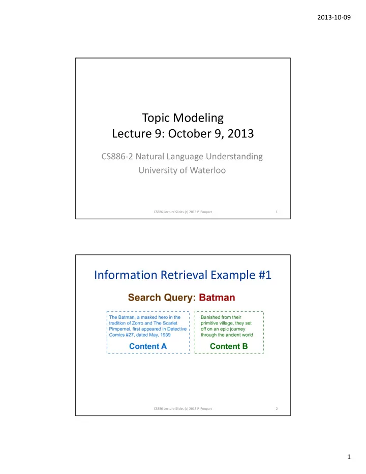
Information Retrieval Example #1
CS886 Lecture Slides (c) 2013 P. Poupart 2