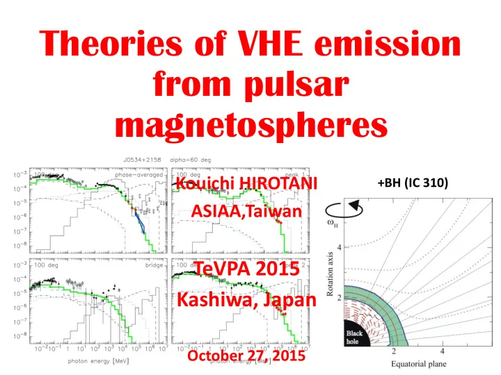
SLIDE 1 Theories of VHE emission from pulsar magnetospheres
Kouichi HIROTANI ASIAA,Taiwan
TeVPA 2015 Kashiwa, Japan
October 27, 2015
+BH (IC 310)
SLIDE 2 §1 g-ray Pulsar Observations
Fermi/LAT point sources (>100 MeV)
Crab Geminga Vela
2nd LAT catalog (Abdo+ 2013)
After 2008, LAT aboard Fermi has detected more than 117 pulsars above 100 MeV.
Large Area Telescope Fermi g -ray space telescope
LAT MSPs LAT radio-loud PSRs LAT radio-quiet PSRs
SLIDE 3 Pulsed broad-band spectra of young pulsars
NS age 103 yrs 105 yrs
High-energy (~GeV) photons are emitted mainly via curvature process by ultra-relativistic, primary e-’s/e+’s. However, > 20 GeV, Inverse-Compton scatterings (ICS) by the cascaded e’s contribute.
100 MeV
Crab B1059-58 Vela B1706-44 B1951+32 Geminga B1055-52
nFn eV hn
(created in particle accelerator) (Thompson, EGRET spectra)
SLIDE 4
§2 Pulsar Emission Models
Where are such incoherent, high-energy photons emitted from pulsars?
SLIDE 5
§2 Pulsar Emission Models
If copious charges are (somehow) supplied, they realize a force-free magnetosphere, E·B=0, and corotate with the magnetosphere under the corotational electric field, 𝑭⊥ ≡ −𝑑−1(𝜵 × 𝒔) × 𝑪. Charges corotate by 𝑭⊥ × 𝑪 drift, 𝒘j ≡ 𝜵 × 𝒔.
SLIDE 6
§2 Pulsar Emission Models
If copious charges are (somehow) supplied, they realize a force-free magnetosphere, E·B=0, and corotate with the magnetosphere under the corotational electric field, 𝑭⊥ ≡ −𝑑−1(𝜵 × 𝒔) × 𝑪. But 𝑭⊥ cannot accelerate charged particles. In 𝛼 · 𝑭 = 4𝜌𝜍, we set E = E^ + Enon-corotate , to obtain 𝛼 · 𝑭⊥ + 𝑭non−corotate = 4𝜌𝜍, that is, 𝛼 · 𝑭non−corotate = 4𝜌(𝜍 − 𝜍GJ), where 𝜍GJ≡ 𝛼 · 𝑭⊥/4𝜌~ − 𝜵 · 𝑪/2𝜌𝑑. If r deviates from rGJ in some region, E|| =𝑭non−corotate · 𝑪/B arises around that region.
SLIDE 7 §2 Pulsar Emission Models
If copious charges are (somehow) supplied, they realize a force-free magnetosphere, E·B=0, and corotate with the magnetosphere under the corotational electric field, 𝑭⊥ ≡ −𝑑−1(𝜵 × 𝒔) × 𝑪. But 𝑭⊥ cannot accelerate charged particles. In 𝛼 · 𝑭 = 4𝜌𝜍, we set E = E^ + Enon-corotate , to obtain 𝛼 · 𝑭⊥ + 𝑭non−corotate = 4𝜌𝜍, that is, 𝛼 · 𝑭non−corotate = 4𝜌(𝜍 − 𝜍GJ), where 𝜍GJ≡ 𝛼 · 𝑭⊥~ − 𝜵 · 𝑪/2𝜌𝑑. If r deviates from rGJ in some region, E|| =𝑭non−corotate · 𝑪/B arises around that region.
Thus, the problem reduces to …
“Where does the charge deficit (|𝜍| < |𝜍GJ|) arise?”
SLIDE 8
§3 Pulsar Outer gap model
If E|| appears in some region, the accelerator (or the gap) boundaries should connect to the force-free magnetosphere outside, i.e., r=rGJ. Thus, gap appears across a null charge surface, where rGJ=0.
SLIDE 9 §3 Pulsar Outer gap model
In pulsar magnetospheres, null-charge surfaces (rGJ=0) appear due to the global curvature of a dipole B field. Null surfaces appear in the higher altitudes (near the light cylinder, ~102 RNS), because the open B lines
- ccupies very small area,
- n the NS surface.
Null-charge surface Light cylinder Outer gap
𝜍GJ≡ 𝛼 · 𝑭⊥/4𝜌~ − 𝜵 · 𝑪/2𝜌𝑑
SLIDE 10 §3 Pulsar Outer gap model
As a model of high-altitude emissions, we investigate the
Cheng, Ho, Ruderman (1986, ApJ 300, 500)
Emission altitude ~ light cylinder hollow cone emission (DW > 1 ster) OG model was further developed by including special relativistic effects.
Romani (1996, ApJ 470, 469)
Successfully explained wide- separated double peaks. OG model became promising.
SLIDE 11
§3 Outer-gap Model: Formalism
e’s are accelerated by E|| Relativistic e+/e- emit g-rays via synchro-curvature, and IC processes g-rays collide with soft photons/B to materialize as pairs in the accelerator I quantify the classic OG model by solving the pair- production cascade in a rotating NS magnetosphere:
SLIDE 12 §3 Outer-gap Model: Formalism
2 2 2 2 GJ 2 2 2 GJ ion 1
4 ( ) , where , , 2 ( ) ( , , ) ( , , ) + ( ), ( , , ) . x y z E x c e d d N N x y z
r r r r g g g r
Ω B x x x x x
Poisson equation for electrostatic potential ψ : N+/N-: distrib. func. of e+/e- g : Lorentz factor of e+/e- : pitch angle of e+/e-
SLIDE 13 §3 Outer-gap Model: Formalism
Assuming t+Wf =0 , we solve the e’s Boltzmann eqs. together with the radiative transfer equation, N: positronic/electronic spatial # density, E||: mangnetic-field-aligned electric field, SIC: ICS re-distribution function, dw: solid angle element, In: specific intensity, l : path length along the ray an: absorption coefficient, jn: emission coefficient
IC SC
N t I N v v N eE B S S d d c h p
n n
a n w n
dI I j dl
n n n n
a
SLIDE 14
§4 OG model: the Crab pulsar
Next, we apply the scheme to the Crab pulsar. Recent force-free, MHD, and PIC simulations suggest that B field approaches a split monopole (Michael’74) near and beyond the light cylinder. Thus, we consider B= vacuum, rotating dipole B + b × split-monopole B b=0: pure dipole b=1: Bdipole=Bmonopole @ LC
SLIDE 15 §4 OG model: the Crab pulsar
3-D distribution of the particle accelerator (i.e., high- energy emission zone) solved from the Poisson eq.:
NS last-open B field lines e-/e+ accelerator
SLIDE 16 §4 OG model: the Crab pulsar
E|| is heavily screened by the produced pairs. → Outward flux » Inward flux (KH ’15, ApJ 798, L40).
Max(E||) are projected on the last-open B surface. 3-D gap solution (non-vacuum)
SLIDE 17 §4 OG model: the Crab pulsar
b=0 (pure rotating vacuum dipole)
0.1-30 GeV >30 GeV (x10)
The resultant g-ray light curves changes as a function of the observer’s viewing angles:
P1 P2 One NS rotation
B inclination: a=65o
Obs.
z
z= z= z= z=
SLIDE 18 §4 OG model: the Crab pulsar
b=0 (pure rotating vacuum dipole) b=0.5 (dipole + weak monopole) b=1.0 (+ moderate monopole) b=2.0 (+ strong monopole)
a=65o
P1 P2 0.1-30 GeV >30 GeV (x10)
SLIDE 19 §4 OG model: the Crab pulsar
b=0 (pure rotating vacuum dipole) b=0.5 (dipole + weak monopole) b=1.0 (+ moderate monopole) b=2.0 (+ strong monopole)
P1/P2 increases as B approaches monopole. P1/P2 decreases with increasing photon energy. From P1/P2 behavior, a weak superposition of monopole is preferable. I.e., the true solution of B will be found between the pure dipole and the force- free solution.
SLIDE 20 §4 OG model: the Crab pulsar
b=0 (pure rotating vacuum dipole) b=0.5 (dipole + weak monopole) b=1.0 (+ moderate monopole) b=2.0 (+ strong monopole)
For very young pulsars like Crab, P2 spectrum gets harder than P1, because gg collision angles are small in TS due to the caustic (aberration+time-of-flight delay) effect.
- Cf. In general, P2 curvature specrum is harder than P1,
because Rc is greater in TS.
(KH ApJ 733, L49, 2011)
SLIDE 21 §4 OG model: the Crab pulsar
Phase-resolved spectrum (Crab, b=0.5, a=65o, z=118o)
Total pulsed P2
SLIDE 22
§4 OG model: the Crab pulsar
Viewing angle dependence: z=95o for b=0 & a=60o
SLIDE 23
§4 OG model: the Crab pulsar
Viewing angle dependence: z=100o for b=0 & a=60o
SLIDE 24
§4 OG model: the Crab pulsar
Viewing angle dependence: z=105o for b=0 & a=60o
SLIDE 25
§4 OG model: the Crab pulsar
Viewing angle dependence: z=105o for b=0 & a=60o 3-D simulation of the outer gap can constrain the viewing angles of individual pulsars.
SLIDE 26 §5 BH gap model
Same method can be applied to BH magnetospheres. The BH gap model itself is applicable to arbitrary BH mass (from stellar-mass to supermassive), spin, and accretion rate (from LLAGN to quasars)
Beskin + (1992, Soviet Ast. 36, 642) KH & Okamoto (1998, ApJ 497, 653)
We present a new method to quantify the previous BH models (Levinson & Rieger 2011, ApJ 730, 123; Broderick &
Tchekhovskoy 2015, ApJ 809, 97).
Today, as an example, we apply the BH gap model to IC310.
KH & Pu (2015, ApJ, submitted)
SLIDE 27 §5 BH gap model
A possible target: IC310 BH lightning due to particle acceleration @ horizon scale
(Science 346, 1080-1084, MAGIC collaboration 2014)
MAGIC observed radio galaxy IC 310 (S0, z =0.0189) on Nov 12-13, 2012. M-s rel.→ M=(1~7)×108 Mʘ, DtBH = 8~57 min. Extraordinary outburst was detected above 300 GeV. Conservative estimate of the shortest variability, Dtobs=4.8 min < (.08-.6)DtBH.
SLIDE 28 §5 BH gap model
BH lightning due to particle acceleration @ horizon scale
(Science 346, 1080-1084, MAGIC collaboration 2014) Mrk 501 & PKS 2155-304 show VHE variabilities with flux doubling times scales, Dtobs ~ 2 min « DtBH. (~70-80 min.)
(Albert + 2007, ApJ 685, L23; Abramowski + 2012, ApJ 746, 151)
Imagine a perturbation initiating in the AGN-rest frame with variation time scale DtAGN. The perturbation enters into the jet with time scale GDtAGN. We detect variation Dtobs=(1+z) (G/d) DtAGN ~ DtAGN. Since G~d, Lorentz factors cancel out in the observer’s frame.
→ D tobs« DtBH indicates variations at sub-horizon scales. If the initial perturbation originates in the AGN-rest frame, the variability takes place at sub-horizon scale.
SLIDE 29 §5 BH gap model
To interpret the sub-horizon phenomena, we apply the pulsar outer-gap model to the BH magnetosphere of IC 310. GR Goldreich-Julian charge density: W: angular frequency of B field w: angular frequency of space-time dragging a: redshift factor (or the lapse function) Y: magnetic flux function, Af. describes In BH magnetosphere, null surface is formed by space- time dragging near the horizon, close to the W=w surface.
GJ
1 4 2 c w r a W Y , 2 2
p p
e c
f
w a Y W Y B E
SLIDE 30 §5 BH gap model
KH & Pu 2015, submitted to ApJ
Distribution of null surface (rGJ=0 due to frame dragging).
Radial B on (r,q) plane Parabolic B on (r,q) plane W=0.3wH W=0.3wH
SLIDE 31 §5 BH gap model
KH & Pu 2015, submitted to ApJ
Gap exits as a solution
- f the set of Poisson
- eq. for Y and e± & g
Boltzmann eqs. E|| arises along B. Frame dragging determines rGJ. Thus, rGJ(r,q) and hence the solution little depends on B (r,q). We thus assume radial B on poloidal plane. Gap distribution for W=0.3wH,
5 Edd
3.2 10 M M
SLIDE 32 §5 BH gap model
KH & Pu 2015, submitted to ApJ
Along B, r ≠rGJ, leading to non- vanishing E||. Example of E||(s) at q =15o (polar funnel).
5 Edd
3.2 10 M M
E||(s) Poisson eq: 𝛼 · E|| = 4𝜌(𝜍 − 𝜍GJ) B=104 G (fixed, not equilibrium)
SLIDE 33 §5 BH gap model: Results
w increases with decreasing . Since Lgap w4, the gap becomes most luminous when the inner boundary almost touches down the horizon.
Edd
/ M M
B=104 G (fixed)
Gap width Decreasing M
w=s2-s1
KH & Pu 2015, submitted to ApJ
SLIDE 34 §5 BH gap model
KH & Pu 2015, submitted to ApJ
Large curvature radius, Rc=10r.
B=104 G (fixed, not equil.)
SLIDE 35 §5 BH gap model
KH & Pu 2015, submitted to ApJ
Small curvature radius, Rc=0.1r.
B=104 G (fixed, not equil.)
SLIDE 36 §5 BH gap model
KH & Pu 2015, submitted to ApJ
Superpose Rc=10r (67%) & Rc=0.1r (33%). Power-law-like SED is formed.
B=104 G (fixed, not equil.)
SLIDE 37 Summary
“Moderate B deformation (b~0.5) near LC is preferable to reproduce P1/P2 ratio and relatively large peak separation. Bridge emission reduces due to strong screening. E|| screening in middle & lower altitudes naturally leads to
- utward-dominated outer-gap emission.
The VHE flare state of IC 310 can be reproduced w/ the BH gap model @ for a=0.998M. The same method can be applied to other low-luminosity AGNs and to (stellar-mass) BH binaries.
6 Edd
4.9 10 M M
SLIDE 38
Summary (cont’d)
E|| sign is opposite between PSR and BH magnetospheres, because a null surface is formed by global B convex geometry in PSRs, but by the frame dragging in BHs. Soft photons are provided by NS surface thermal X-rays in PSR magnetospheres, but by accretion flow in BH ones. Accretion quenches gaps in PSRs, but switches on BHs, because b«1 in PSRs, but b ~1 in BHs. HE/VHE emission is dependent on B geometry in PSRs, but independent in BHs, because null surface is formed by B geometry in PSRs but by frame dragging in BHs.