the time complexity of backprop auto diff and the baur
play

The time complexity of Backprop; Auto-Diff; and the Baur-Strassen - PDF document

CSE 446: Machine Learning Lecture The time complexity of Backprop; Auto-Diff; and the Baur-Strassen theorem Instructor: Sham Kakade 1 Multi-layer perceptrons We can specify an L -hidden layer network as follows: given outputs { z ( l ) j } from


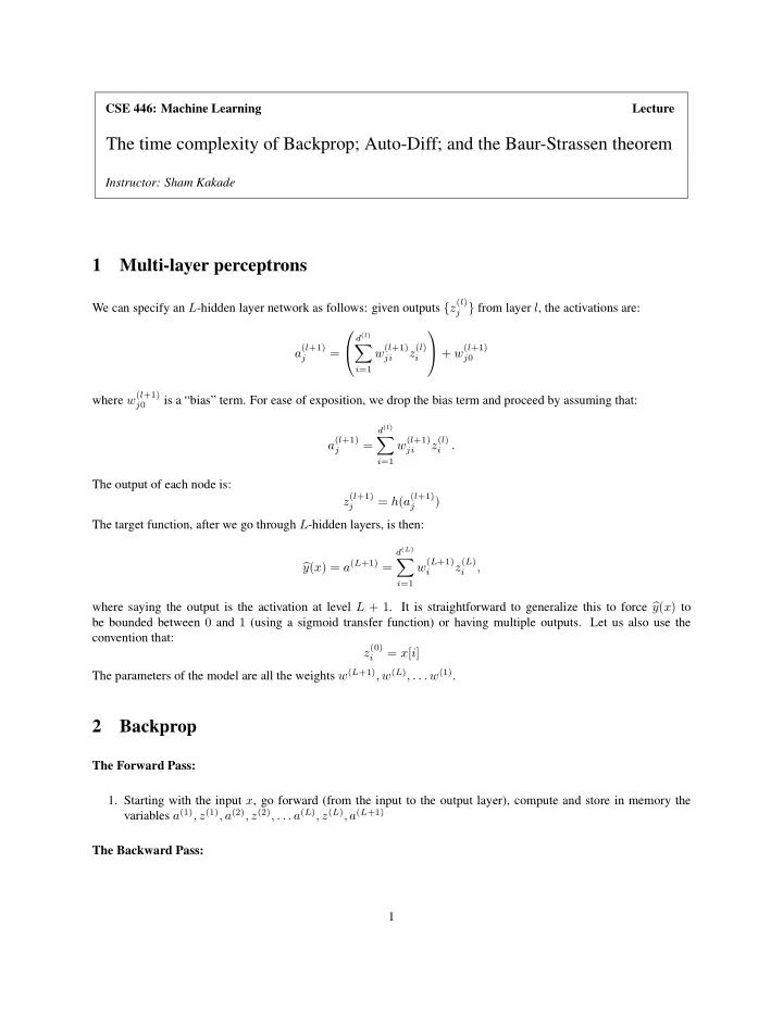
  1. CSE 446: Machine Learning Lecture The time complexity of Backprop; Auto-Diff; and the Baur-Strassen theorem Instructor: Sham Kakade 1 Multi-layer perceptrons We can specify an L -hidden layer network as follows: given outputs { z ( l ) j } from layer l , the activations are:   d ( l ) � a ( l +1) w ( l +1) z ( l )  + w ( l +1)  = j ji i j 0 i =1 where w ( l +1) is a “bias” term. For ease of exposition, we drop the bias term and proceed by assuming that: j 0 d ( l ) � a ( l +1) w ( l +1) z ( l ) = . j ji i i =1 The output of each node is: z ( l +1) = h ( a ( l +1) ) j j The target function, after we go through L -hidden layers, is then: d ( L ) � y ( x ) = a ( L +1) = w ( L +1) z ( L ) � , i i i =1 where saying the output is the activation at level L + 1 . It is straightforward to generalize this to force � y ( x ) to be bounded between 0 and 1 (using a sigmoid transfer function) or having multiple outputs. Let us also use the convention that: z (0) = x [ i ] i The parameters of the model are all the weights w ( L +1) , w ( L ) , . . . w (1) . 2 Backprop The Forward Pass: 1. Starting with the input x , go forward (from the input to the output layer), compute and store in memory the variables a (1) , z (1) , a (2) , z (2) , . . . a ( L ) , z ( L ) , a ( L +1) The Backward Pass: 1
  2. 1. Initialize as follows: δ ( L +1) = − ( y − � y ) = − ( y − a ( L +1) ) and compute the derivatives at the output layer: ∂ℓ ( y, � y ) y ) z ( L ) = − ( y − � j ∂w ( L +1) j 2. Recursively, compute d ( l +1) � δ ( l ) = h ′ ( a ( l ) w ( l +1) δ ( l +1) j ) j kj k k =1 and also compute our derivatives at layer l : ∂ℓ ( y, � y ) = δ ( l ) j z ( l − 1) i ∂w ( l ) ji 2.1 Time Complexity Assume that addition, subtraction, multiplication, and division take “one unit” of time (and let us ignore numerical precision issues). Let us say the time complexity to compute ℓ ( y, � y ( x )) is based on the naive algorithm (which explicitly just computes all the sums in the forward pass). Theorem 2.1. Suppose that we can compute the derivative h ′ ( · ) in an amount of time that is within a constant factor of the time it takes to compute h ( · ) itself (and suppose that constant is 5 ). Using the backprop algorithm, the (total) time to compute both ℓ ( y, � y ( x )) and ∇ ℓ ( y, � y ( x )) — note that ∇ ℓ ( y, � y ( x )) contains # parameter partial derivatives — is within a factor of 5 of computing just the scalar value ℓ ( y, � y ( x )) . Proof. The number of transfer function evaluations in the forward pass is just the number of nodes. In the backward pass, the number of times we need to evaluate the derivative of the transfer function is also just the number of nodes. In the forward pass, note that the total computation time is a constant factor (actually 2 ) times the number weights. To see this, note that to compute any activation, it costs us (one addition and one multiplication) associated with each weight (and that the every weight is only involved in the computation of just one activation). Similarly, by examining the recursion in the backward pass, we see that the total compute time to get all the δ ’s is a constant factor times the number of weights (again there is only one multiplication and one addition associated with each weight). Also, the compute time for obtaining the partial derivatives from the δ ’s is equal to the number of weights. Remark: That we defined the time complexity to be under the “naive” algorithm is irrelevant. If we had a faster algorithm to compute ℓ ( y, � y ( x )) (say through a faster matrix multiplication algorithm or possibly other tricks), then the above theorem would still hold. This is the remarkable Baur-Strassen theorem [1] (also independently stated by [2]). 3 Why auto-differentiation is possible This is an informal discussion for how to think about and understand auto-differentiation and computation graphs. In short, for functions that we can write with arithmetic operations (as opposed to using branching and “if/elseif/then” statements) then there should be automated (and provably fast) procedures to find their derivatives. 2

  3. This is the basic insight being exploited by PyTorch, TensorFlow, Theano, etc... Auto-differentiation (based on the Baur-Strassen theorem) is a remarkably powerful idea, and an understanding of backprop is really all need to undertand these libraries. More generally, the idea behind backprop is really about how to take the derivative of a function written down in a arithmetic circuit , so auto-diff is very general purpose tool (not limited to neural network learning). 3.1 The Baur-Strassen theorem The arithmetic circuit model is the most natural model for how we compute mathematical functions (it consists of the usual add, subtract, multiply, and divide operations). This circuit does not let you compute a function using “if/elseif/then” statements. Note that if you wrote a function with “if” statements then it is not even obvious if your functions is differentiable. The following theorem shows, in essence, why auto-differentiation is possible. Suppose f is a function of d variables, f ( w 1 , w 2 , . . . w d ) . Remarkably, the time to compute both the function and all its d derivatives is with a constant factor (namely 5 ) of computing the functions itself. Theorem 3.1. (“All for the price of one” [1, 2]) Suppose f is a differentiable function which we can compute in the ∂w 1 , ∂f ∂f ∂w 2 , . . . ∂f arithmetic circuit model. Then the time it takes to compute both f and its d partial derivatives ∂w d is within a factor of 5 of the time it takes to compute just f . Proof. (the basic idea) The idea of the proof is really that we can view a circuit as just a type of neural network. And then the proof is really just the same as that of the backprop proof we just did! 3.2 Auto-differentiation and Computation Graphs One way to think about computation graphs is that they are analogous to how a neural net computes your function: the basic idea is that, looking at the structure in your code (say, as it is being run), it should be possible to just build the underlying “circuit” on the fly (this is the “computation graph”). And then the backward pass can be done automatically using this graph. With some libraries like TensorFlow, you have to be more explicit about the computation graph. Basically, we can think that the “nodes” in the computation graph corresponding to the intermediate variables that we create along the way when we are defining how to compute our function. Note that we have to be doing arithmetic for this approach of auto-differentiation to make any sense. In contrast, if we have an “if” statement in our function, it is far from obvious how we can “auto-differentiate” this function (or even if the derivative exists). References [1] Walter Baur and Volker Strassen. The complexity of partial derivatives. Theoretical Computer Science , 22:317– 330, 1983. [2] Andreas Griewank and Andrea Walther. Evaluating Derivatives: Principles and Techniques of Algorithmic Dif- ferentiation . Society for Industrial and Applied Mathematics, Philadelphia, PA, USA, second edition, 2008. 3

Download Presentation
Download Policy: The content available on the website is offered to you 'AS IS' for your personal information and use only. It cannot be commercialized, licensed, or distributed on other websites without prior consent from the author. To download a presentation, simply click this link. If you encounter any difficulties during the download process, it's possible that the publisher has removed the file from their server.

Recommend


More recommend