The Specialist Committee on Uncertainty Analysis Final Report and - - PDF document

433

Proceedings of 25th ITTC – Volume II

The Specialist Committee on Uncertainty Analysis

Final Report and Recommendations to the 25th ITTC

• 1. INTRODUCTION

1.1 Membership and Meetings The uncertainty analysis committee (UAC) was appointed by the 24th ITTC in Edinburgh, Scotland, 2005, and it consists of the following members shown in Figure 1:

• Dr. Joel T. Park (Chairman): Naval Surface

Warfare Center Carderock Division, NSWCCD, West Bethesda, Maryland, USA.

• Dr. Ahmed Derradji-Aouat (Secretary):

National Research Council Canada, Insti- tute for Ocean Technology, NRC-IOT, Newfoundland and Labrador, Canada.

• Mr. Baoshan Wu: China Ship Scientific

Research Centre, CSSRC, Wuxi, Jiangsu, China.

• Dr. Shigeru Nishio: Kobe University, Fac-

ulty of Maritime Sciences, Department of Maritime Safety Management, Kobe, Japan.

• Mr. Erwan Jacquin: Formerly a staff mem-

ber of the Bassin d’Essais des Carènes, BEC, Val-de-Reuil, France. Four (4) UAC meetings were held. The host Countries, host laboratories, and dates of the meetings were:

• France, BEC, March 30-31, 2006.
• China, CSSRC, October 23-25, 2006.
• Canada, NRC-IOT, June 7-8, 2007.
• USA, NSWCCD, January 30-February 1,

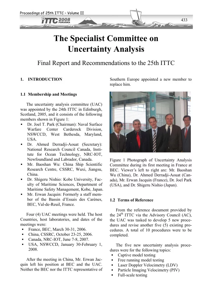
2008. After the meeting in China, Mr. Erwan Jac- quin left his position at BEC and the UAC. Neither the BEC nor the ITTC representative of Southern Europe appointed a new member to replace him. Figure 1 Photograph of Uncertainty Analysis Committee during its first meeting in France at

• BEC. Viewer’s left to right are: Mr. Baoshan

Wu (China), Dr. Ahmed Derradji-Aouat (Can- ada), Mr. Erwan Jacquin (France), Dr. Joel Park (USA), and Dr. Shigeru Nishio (Japan). 1.2 Terms of Reference From the reference document provided by the 24th ITTC via the Advisory Council (AC), the UAC was tasked to develop 5 new proce- dures and revise another five (5) existing pro-

• cedures. A total of 10 procedures were to be

completed. The five new uncertainty analysis proce- dures were for the following topics:

• Captive model testing
• Free running model testing
• Laser Doppler Velocimetry (LDV)
• Particle Imaging Velocimetry (PIV)
• Full-scale testing

434

The Specialist Committee on Uncertainty Analysis

Since the UAC started with only with 5 members, the departure of Mr. E. Jacquin from the BEC, France, led to the decision to elimi- nate the work for full-scale testing. Addition- ally, future full-scale test procedures may be derived from the procedures on captive and free-running model tests. The five existing uncertainty analysis pro- cedures that were to be revised are as follows:

• 7.5-02-01-01 Uncertainty Analysis in EFD,

Uncertainty Assessment Methodology (19 pages)

• 7.5-02-01-02 Uncertainty Analysis in EFD,

Guidelines for Resistance Towing Tank Tests (5 pages)

• 7.5-02-03-01.2 Propulsion, Performance

Uncertainty Analysis, Example for Propul- sion Test (26 pages)

• 7.5-02-03-02.2 Propulsion, Propulsor Un-

certainty Analysis, Example for Open Wa- ter Test (15 pages)

• 7.5-02-07-03.2 Testing and Extrapolation

Methods Loads and Responses, Ocean En- gineering Analysis Procedure for Model Tests in Regular Waves (8 pages). ITTC procedure 7.5-02-07-03.2 did not have an uncertainty component; therefore, nothing was available to review. The UAC may provide a document to the appropriate commit- tee so it can be added to that existing procedure. During the first meeting in France, the UAC concluded that ITTC 7.5-02-01-02 could be eliminated since it provided no new informa- tion in support of ITTC 7.5-02-01-02. The UAC subsequently submitted two revised pro- cedures, ITTC (2008a, b). More importantly, during the first meeting in France, the UAC de- cided to adopt a more inclusive philosophy and follow the guidelines of the ISO (1995), also known as ISO-GUM (Guide to the Expression

• f Uncertainty in Measurements).

Application of the ISO (1995) to experi- mental hydrodynamics is a fundamental shift in thinking and in assessing uncertainties from what the ITTC historically had followed. Up to the 24th ITTC in 2005, the ITTC opted for the method of AIAA (1995), which was revised as AIAA (1999) for the development of ITTC UA

• procedures. AIAA (1999) is for wind tunnel
• testing. The UA standards for wind tunnel test-

ing were considered applicable to experimental hydrodynamics and tow tank testing. Starting in 2005 just after the creation of the UAC during the 24th ITTC, ITTC member or- ganizations from geographic areas other than North America have demanded the use of ISO (1995) rather than AIAA (1999) or ASME (2005). Both AIAA and ASME are American

• rganizations, and ISO was viewed as the le-

gitimate international organization for guides and standards development. Since the procedures for development by the UAC should be consistent with ISO (1995), the review of the 3 procedures 7.5-02-03-01.2, 7.5-2-03-02.2, and 7.5-02-07-03.2 were post- poned after completion of ITTC (2008a). The development of the 2 new procedures on LDV and PIV were possible because the committee members were specialists in the subject areas as well as in ISO (1995). An uncertainty analysis procedure for free- running model testing was not developed. In- stead, the UAC provides an example on the ap- plication of uncertainty analysis to free-running models in section 12 of this report. As a consequence for adoption of the ISO (1995) as the basis of ITTC (2008a), all exist- ing and recommended ITTC UA procedures should be reviewed and revised accordingly. The 26th ITTC General and Specialist Commit- tees should harmonize their existing UA proce- dures with ITTC (2008a). Any new UA proce- dures should also follow this new procedure as

• well. The UAC will provide assistance and

guidance to various ITTC committees for har- monization of their existing and new proce-

• dures. Since ISO (1995) is concerned only with

general guidelines for expressing uncertainties in measurements, specific disciplines such as experimental hydrodynamics should produce

435

Proceedings of 25th ITTC – Volume II

specific UA procedures and show how the ISO (1995) guidelines are implemented. 1.3 Additional Activities The UAC proposed a new procedure on in- strument calibration, ITTC (2008c). Although the ITTC terms of reference did not include a mandate for such a procedure, a procedure for UA Instrument Calibration is a fundamental extension to the general procedure (ITTC, 2008a). In addition to the AC mandated tasks, the UAC played a proactive role in interacting and discussing UA related issues with other ITTC

• committees. Among these committees are the

Specialist Committee on Powering, Perform- ance Prediction, the Propulsion Committee, the Manoeuvring Committee, Resistance Commit- tee, and the Seakeeping Committee. Some lim- ited discussions with members of the Specialist Committee on Ice took place. 1.4 Symbols and Definitions The basic and general definitions for me- trology terms in ITTC (2008a) are the same as those given by the International Vocabulary for Metrology (VIM, 2007). This is also an ISO publication from the Bureau International des Poids et Mesures (BIPM) that is complimentary to the ISO (1995). Among these, are definitions for terms such as “measurand”, “measurement”, “error”, “uncertainty”, “repeatability”, “repro- ducibility”, and other expressions routinely mentioned in ISO (1995).

• 2. COMPLETED PROCEDURES

Five procedures were completed by the UAC, all based on ISO (1995) guidelines. The five procedures are:

• 7.5-02-01-01. Guide to the Expression of

Uncertainty in Experimental Hydrodynam- ics.

• 7.5-02-01-02. Guidelines for Uncertainty

Analysis in Resistance Towing Tank Tests.

• 7.5-01-03-01. Uncertainty Analysis: In-

strument Calibrations.

• 7.5-01-03-02. Uncertainty Analysis: Laser

Doppler Velocimetry (LDV).

• 7.5-01-03-03. Uncertainty Analysis: Parti-

cle Imaging Velocimetry (PIV).

• 3. STRUCTURE OF THE REPORT

This document is divided into four sections:

• Uncertainty Analysis section that includes

general literature for the UA, its history, its importance, and why it is needed.

• Summary for the new and revised proce-

dure completed by the UAC.

• Other activities section that includes inter-

actions with other ITTC committees, dis- cussion of UA application to free running model tests, and UA in fundamental equa- tions for water properties (density, viscos- ity and vapour pressure).

• Conclusions and recommendations.
• 4. UNCERTAINTY ANALYSIS

4.1 Brief History of Uncertainty Analysis Modern uncertainty analysis in North America evolved from a series of papers pub- lished by professors and their students from Stanford University, S. R. Kline, R. J. Moffat, and H. W. Coleman. The earliest paper was by Kline and McKlintock (1953). They introduced concepts such as single sample uncertainty, un- certainty interval, and the law of propagation of

• uncertainty. Kline and McKlintock (1953) also

suggested describing the uncertainty with 20 to 1 odds. In current practice, uncertainty esti- mates are stated at the 95 % confidence level rather than 20 to 1 odds, which are equivalent. In the international community, a group of experts formulated recommendation INC-1 (1980) “expression of uncertainty in measure-

436

The Specialist Committee on Uncertainty Analysis

ments” under the sponsorship of Le Bureau In- ternational des Poids et Mesures (BIPM). His- torically the creation of the BIPM goes back to Convention of the Metre (Convention du Mètre) 1875, 17 member nations signed a treaty in Paris (now that number is 51 nations are members and 27 states are associate mem- bers). The treaty, signed in 1875, gives author- ity to the General Conference on Weights and Measures (CGPM), the International Commit- tee for Weights and Measures (CIPM) and the International Bureau of Weights and Measures (BIPM) to act in matters of world metrology, particularly concerning the demand for meas- urement standards of ever increasing accuracy, range and diversity, and the need to demon- strate equivalence between national measure- ment standards. The recommendation INC-1 (1980) became the basis of the ISO (1995), which was first published in 1993. The text for the recommen- dation INC-1 (1980) is included the ISO (1995) in both French (original text) and English and Giacomo (1981). At the BIPM, the ISO (1995) is the respon- sibility of the Working Group on the Expres- sion of Uncertainty in Measurement (GUM), which is also known as Working Group 1 (WG1). WG1 is one of 2 working groups within the Joint Committee for Guides in Me- trology (JCGM). The second working group (WG2) is responsible for the International Vo- cabulary of Basic and General Terms in Me- trology, known as the VIM. The JCGM took the responsibility for both GUM and VIM documents from ISO TAG 4 (Technical Advi- sory Group 4). In the near future, the JCGM does not anticipate any revisions to the ISO (1995), but is in the process of providing sup- plements. 4.2 Basic Principles for the ISO GUM 1995 Uncertainty Analysis Guideline The original concepts for the expression of uncertainty analysis were relatively simple and are summarized in the following 5 principles Giacomo (1981) and ISO (1995): Principle 1. The uncertainty results may be grouped in 2 categories called Type A uncer- tainty and Type B uncertainty. They are de- fined as follows:

• Type A uncertainties are those evaluated

by applying statistical methods to the re- sults of a series of repeated measurements.

• Type B uncertainties are those evaluated

by other means. The definition has been further refined by ISO (1995) to include prior experience and professional judg- ments, manufacturer’s specifications, pre- vious measurement data, calibrations, and reference data from handbooks. Pre-GUM methodologies, the methodolo- gies developed prior to ISO (1995), also clas- sify total uncertainty into two components “random and systematic” in ASME 19.1-2005

• r “precision and bias” in AIAA (1999).

No simple correspondence exists between the classification categories A and B and the classifications of the Pre-GUM methodologies. Recommendation INC-1 (1980) indicated that the term ‘systematic uncertainty’ can be mis- leading and should be avoided”. ASME PTC 19.1-2005 has retained the terms “systematic” and “random” and avoided intentionally the use

• f terms “bias” and “precision”.

Principle 2. The components in type A un- certainty are defined by the estimated variance, which includes the effect of the number of de- grees of freedom (DOF). Principle 3. The components in type B un- certainty are also approximated by a corre- sponding variance, in which its existence is as- sumed. Principle 4. The combined uncertainty should be computed by the normal method for the combination of variances, now known as the law of propagation of uncertainty.

437

Proceedings of 25th ITTC – Volume II

Principle 5. For particular applications, the combined uncertainty should be multiplied by a coverage factor to obtain an overall uncertainty

• value. The overall uncertainty is now called

expanded uncertainty. For the 95 % confidence level, the commonly applied coverage factor is 2. 4.3 Pre-GUM Methodologies The term Pre-GUM refers to methodologies developed prior to ISO (1995). Moffat (1982) introduced and defined the terms “bias” and “precision”. The jitter diagram was proposed as a computational tool to propagate uncertainties by a central finite differencing method. This method is now included in the ISO (1995), sec- tion 5.1.3 on p. 19. Moffat (1985) also introduced the term rela- tive uncertainty for equations containing prod- ucts of the terms (see equation 12, section 5.1.6,

• p. 20 of the ISO, 1995). Typical examples for

such equations in experimental hydrodynamics are Reynolds number, Re, and Froude number, Fr. The developmental progress of the uncer- tainty methodology in North America was de- scribed in a series of four (4) papers published in 1985: Abernethy and Benedict (1985), Kline (1985), Abernethy, et al. (1985), and Moffat (1985). The last 3 papers were originally pre- sented in the Symposium on Uncertainty Analysis at the Winter Annual Meeting of the American Society of Mechanical Engineers (ASME) in Boston in 1983. The following is a brief discussion regard- ing Pre-GUM schools of thought or standards. The focus is on two particular USA standards, ASME (2005) and AIAA (1999). ASME PTC 19.1 was first published in 1985, since then, PTC 19.1 has been updated and revised twice. The last two revisions ASME PTC 19.1-1998 and ASME PTC 19.1- 2005 are in harmony with the ISO (1995). The term “harmonization” employed by AMSE does not mean the same equations and same

• process. Harmonization is rather the manner

how uncertainty analysis is assessed. The ASME PTC 19.1 series (1985, 1998, and 2005) provided the mathematics necessary to calculate the two components of uncertainty. In ASME 1998, the terms “bias uncertainty” and “precision uncertainty” were applied. However, in ASME 2005, the terms “bias un- certainty” and “precision uncertainty” were in- tentionally avoided and replaced by “system- atic” and “random” uncertainties. In ASME PTC 19.1-1998, the term “total uncertainty” is defined, and at the 95 % confi- dence level the total uncertainty (Ut) is given by: (1a) where B is the propagated bias uncertainty from the measurement, S is the propagated pre- cision uncertainty, and t95 is the inverse Student t at the 95 % confidence level. In ASME 19.1-2005, equation (1a) was

• changed. The term “combined uncertainty” has

replaced the term “total uncertainty”. Equation (1a) then becomes for the standard uncertainty: (1b) where b = B/2 and s are the systematic uncer- tainty component and the random uncertainty components, respectively. Also in ASME (2005), the term “expanded uncertainty”, U (Capital U), is defined as: (2) where the coverage factor is 2 for the 95% con- fidence level.

( )

2 95 2 2 t

S t B U + =

2 2 2

s b u + = u U 2 =

438

The Specialist Committee on Uncertainty Analysis

Moffat (1988) provided a practical guide to engineering application of uncertainty analysis. He describes in detail the process from calibra- tion of instrumentation to the analysis of the final experimental results. The bias component consisted of those from calibration, data acqui- sition, and data reduction, components that produce constant uncertainty value during test-

• ing. Acquisition of data during calibration with

modern data acquisition systems includes some precision terms, but the calibration data be- comes a fixed number when applied to the data analysis of the final experimental results. Mof- fat (1988) refers to this constant uncertainty as “fossilized uncertainty”. Coleman and Steele (1999) is the com- monly used textbook on uncertainty analysis by the North American scientists and engineers. The first edition was published in 1989. H. W. Coleman was a USA representative on the committee for AGARD AR-304 (1994). AGARD (1994) was an international effort in the application of uncertainty analysis to wind tunnel testing, which was published a year after the first version of ISO in 1993. In AGARD (1994), total uncertainty was described by an equation similar to equation (1b) as follows: (3) where Bf is the bias uncertainty and Pf the pre- cision uncertainty for the propagated uncer- tainty for the function f or data reduction equa- tions. The law for propagation of uncertainty was expanded by AGARD (1994) for inclusion of perfectly correlated terms. ASME PTC 19.1- 1998 also included relationships for perfectly correlated terms. However, ISO (1995) in- cluded a generalized law of propagation of un-

• certainty. The general propagation law ac-

counts for any correlation term, from which the perfectly correlated version can be derived (see new procedure ITTC (2008a). AIAA S-071A-1999 and its supplement AIAA G-045-2003 are derived from AGARD AR-304 (1994). ITTC uncertainty procedures were previously adapted from the AIAA (1995) version of AIAA S-071. Like ASME PTC 19.1-1998, AIAA S-071A-1999 has been har- monized with ISO (1995). In open literature, both AIAA and ASME standards are quite ex- tensive, have many examples, and are refer- ences useful to ITTC UA procedure develop- ment. In 1993, the National Institute of Standards and Technology (NIST, www.nist.gov/) pub- lished an abbreviated version of ISO (1995). NIST is the National Metrology Institute (NMI) in the USA. The NIST technical note 1297 was revised in 1994 (Taylor and Kuyatt, 1994). Technical Note 1297 is an outline of the im- plementation of ISO (1995) by NIST. Founded in 1901, NIST is a non-regulatory federal

• agency. Its mission is to promote U.S. innova-

tion and industrial competitiveness by advanc- ing measurement science, standards, and tech- nology in ways that enhance economic security and improve our quality of life. Expanded uncertainty is acknowledged as the reporting method for commercial, industrial, and regulatory applications. AIAA (1999) rec-

• mmends traceability of calibrations to an NMI

such as NIST. However by Taylor and Kuyatt (1994), NIST reports uncertainty as standard

• uncertainty. Like the NIST and its technical

note 1297, the ITTC UAC provided general procedures ITTC (2008a, c) as examples of im- plementation of ISO (1995) concepts in ex- perimental hydrodynamics and instrument cali- bration in tow tank and water tunnel testing. ITTC UAC recommended policy is reporting expanded uncertainty at the 95 % confidence level. 4.4 Road to Harmonization The ASME (2005) revision of the PTC 19.1 is written with the objective to harmonize it with the ISO (1995). ISO (1995) recommends

2 2 2 f f f

P B U + =

439

Proceedings of 25th ITTC – Volume II

an expanded uncertainty at the 95 % confi- dence level in industrial applications while ASME PTC 19.1-2005 requires 95 % confi- dence level in reporting expanded uncertainty. The terms “combined uncertainty and ex- panded uncertainty” are applied in both stan-

• dards. Both standards ASME PTC 19.1-2005

and ISO (1995) employ the term standard un- certainty, which is equivalent to one standard deviation. However unlike ISO (1995), ASME PTC 19.1 emphasizes the following fundamental concept: The effect on the final test results de- termines the type of the uncertainty component. Systematic uncertainty component is from error sources whose effect is constant during the ex-

• periment. Random uncertainty component,

however, is from error sources that cause scat- ters in the final results of the experiment. ISO (1995) is based on the fundamental concept that uncertainty components (Type A and Type B) are classified on the method of

• computation. Type A uncertainty is computed

as the standard deviation of the mean value of a series of measurements. However, Type B un- certainty is estimated from other methods, such as previous experience and engineering judg- ment including previous measurement data, calibration data, and manufacturing specifica- tions. ASME PTC 19.1-2005 did not use the terms “bias” and “precision” uncertainty com- ponents as ASME (1998). Instead the terms “systematic error” and “random error” are im-

• plemented. The AIAA (1999) still prefers the

terms “bias” and “precision”. The road to full harmonization among stan- dards is proven to be a difficult and long. NCSLI www.ncsli.org/index.cfm in its PR 12 document (2008) gave a comprehensive com- parison between GUM and Pre GUM standards. No Post-GUM methodologies have been de- veloped independent of ISO (2005). Nations follow ISO (1995), and the US organizations are working to harmonize their standards with that of the ISO (1995). 4.5 Importance of Uncertainty Analysis The importance of uncertainty analysis in science and engineering has been described previously by a number of authors including AGARD (1994), AIAA (1999), Kline (1985), and Coleman and Steele (1999). Kline (1985)

• utlined 12 uses of uncertainty analysis and

provided 7 case histories. The important con- siderations for ITTC are as follows. Data Quality. Uncertainty analysis provides a measure of the quality of the data. Results may be compared between 2 or more laborato- ries or between repeat tests within the same

• laboratory. The results are comparable only if

they are within the uncertainty of the measure-

• ment. Likewise, computational results may be

compared to experimental results. The compu- tational results will be valid only if they are within the uncertainty of the experiment. As a measure of the quality of the data, science and engineering journals as well clients are now requiring an uncertainty statement for the ex- perimental and computational results. In par- ticular, the ASME Journal of Fluids Engineer- ing requires an uncertainty statement for all published papers. Planning an Experiment. Uncertainty analy- sis is necessary for planning of an experiment, and/or improving the results of future experi-

• ments. Pre-test uncertainty analysis will iden-

tify the quality of the instrumentation needed for acquisition of the desired experimental re-

• sults. In most experiments, the uncertainty is

dominated by one or two sources (or instru- ments). Thus, pre-test uncertainty analysis will prevent investment in expensive instruments that do not impact the results significantly. In some cases, an uncertainty analysis will indi- cate that the desired results cannot be achieved and that the experiment should be abandoned. Kline (1985) cites an example of “A Hopeless Experiment Avoided”.

440

The Specialist Committee on Uncertainty Analysis

Diagnostic Tool. Uncertainty analysis can be used as a diagnostic tool. In the planning stage of an experiment, uncertainty analysis will be used to identify major sources of uncer- tainties, why those sources exist, and devise methods for minimization of their effects. Decision Mechanism. Uncertainty analysis can be applied as a decision mechanism. For example, a decision may be necessary for minimization of the effects of a major uncer- tainty source in an experiment. The need for a different load sensor may be driven by the de- sire for a reduction in the overall uncertainty. On the other hand, the new load sensor may be too expensive to buy. Therefore, the decision may be to keep the existing load sensor and ac- cept the pre-calculated level of uncertainty. Uncertainty Growth. Uncertainty growth is new concept that is introduced in the NCSLI PR 12, how uncertainty grows with time for a given component or a sensor (aging factors). The projected uncertainty growth has a direct impact on instrument inventories in the labora- tory and facility operating budgets. Better Understanding. Uncertainty analysis will provide a better understanding of the de- tails and the execution of an experiment. It will provide focus and special care in the acquisi- tion of critical data. Simply said, Kline (1985)

• n the basis of 30 years of laboratory experi-

ence states that uncertainty analysis is worth doing.

• 5. REPEATABILITY VERSUS

REPRODUCIBILITY 5.1 Repeatability In the conventional application of uncer- tainty analysis, uncertainty is estimated from a single test or experiment from single-sample uncertainty theory. In some cases, uncertainty is underestimated due to missing or uncon- trolled elements in the analysis. Detection of such uncontrolled elements may be determined from repeat tests. From ISO (1995), repeatability is defined as “closeness of the agreement between results of successive measurements of the same meas- urand carried out under the same conditions of measurement”. Repeatability conditions are further defined as follows:

• Same measurement procedure
• Same observer/operator
• Same measuring instrument under the

same conditions

• Same location or same laboratory
• Repetition over a short period of time. For

experimental hydrodynamics, a short pe- riod of time may be tests performed on the same day. As an example, repeat tests of carriage speed are illustrated in Figure 2. For laboratory A, the estimated uncertainty in carriage speed from the traditional metal wheel device is indi- cated by the error bars on the symbols. The ex- panded uncertainty in speed was estimated as ±0.00052 m/s or ±0.52 mm/s, at the 95 % con- fidence limit. The mean carriage speed from repeat runs is 2.0375 ±0.0014 m/s, ±0.069 %, with a coverage factor of 2.07. The expanded uncertainty from the repeatability test and metal wheel is then ±0.0015 m/s (±0.074%).

Test Sequence Number

5 10 15 20 25

(V - <V>)/<V> (%)

• 0.15
• 0.10
• 0.05

0.00 0.05 0.10 0.15

Lab A: 2.0375 +/-0.0014 m/s Lab B: 2.54903+/-0.00048 m/s Lab A (2001) Lab B (2006) +/-95% Confidence, A +/-95 % Confidence, B

Figure 2 Comparison of repeatability between carriage speeds of 2 towing basins.

441

Proceedings of 25th ITTC – Volume II

The second data series in Figure 2 is from a second laboratory, laboratory B. In that case, the result for 10 repeat runs was 2.54903 ±0.00048 m/s (±0.019 %) with a coverage fac- tor of 2.26. The uncertainty in the speed meas- urement for Laboratory B is smaller than that from Laboratory A. For laboratory B, the un- certainty in the reference speed was not re- ported, but it is assumed to be similar to that of Laboratory A. The difference in results be- tween the 2 laboratories is probably the control system for carriage speed. No uncertainty esti- mate is likely possible for the contribution of the control system. Consequently, any state- ment on uncertainty in carriage speed for Labo- ratory A should include repeatability in car- riage speed. The estimate stated here is for a single measurement of the carriage speed that is based upon one standard deviation from mul- tiple speeds in the repeat tests. Another example of uncertainty from re- peatability of an experiment is wave height

• measurement. The calibration result for an ul-

trasonic wave height gage from Chirozzi and Park (2005) is shown in Figure 3. Calibration results in Figure 3 are presented as residuals, where a residual is the difference between the data point and its value from a straight-line curve fit. The zero line in Figure 3 represents linear regression value. Further discussion of instrument calibration is in section 8. In this case, calibration of the wave gage is accomplished by relocation of the sensor rela- tive to the water on a shaft with precision pin- hole locations with an estimated uncertainty of ±0.13 mm at the 95 % confidence limit. This uncertainty is smaller than the symbols in the

• figure. The dashed lines in the figure are the

uncertainties at the 95 % confidence level from calibration theory, ITTC (2008c). As the figure indicates, the estimated uncertainty in calibra- tion is within ±4.1 mm. The wave gage is highly linear with an SEE = 0.81 mm (standard error of estimate) and correlation coefficient of r = 0.999993. Since these measurements were acquired by relocation of the sensor relative to the water, the slope and intercept will have signs opposite to those of the calibration for the water surface moving relative to the fixed sen- sor.

Reference Length (mm)

• 400 -300 -200 -100

100 200 300 400

Wave Height Residuals (mm)

• 10
• 8
• 6
• 4
• 2

2 4 6 8 10

Sinex S/N 5740 Intercept: -359.4 mm Slope: +76.40 mm/V SEE: 0.81 mm r: 0.999993 +/-95 % Confidence Limit Wave Height Gage Data

Figure 3 Residual plot of ultrasonic wave gage calibration from Chirozzi and Park (2004). An actual wave measurement from the Ma- noeuvring and Seakeeping Basin (MASK) at David Taylor Model Basin (DTMB) is shown in Figure 4 for regular gravity waves with wave gage #6. The data are unpublished results from a test on March 11, 2004. The total run time was 42.2 s. Only 10 s of data are presented for

• clarity. The red symbols are outliers that were

excluded from a linear regression analysis indi- cated by the solid red line in the figure. A linear regression analysis was performed with a commercial curve fitting code with out- liers removed. For execution of the code, the frequency was fixed with the value from the Fourier analysis. The form of the equation was as follows: (4) where a, b, and c are constants from the regres- sion analysis, and f is the frequency from the Fourier analysis. The results are summarized in Table 1. ) 2 ( c f sin b a y + + = π

442

The Specialist Committee on Uncertainty Analysis

Time (s)

2 4 6 8 10

Wave Height (mm)

• 400
• 300
• 200
• 100

100 200 300 400

Run #1496 11 Mar 2004 Curve Fit Senix Gage #6 Data Outlier Data

Figure 4 Regular wave as measured with an ultrasonic wave height gage. Table 1 Summary of results for regular waves from regression analysis. Symbol Units Value Std Error a mm 11.8 1.58 b mm

• 201.0

2.06 c rad

• 5.253

0.0122 f Hz 0.623 r 0.967 SEE mm 40.3 Thus, the uncertainty in the amplitude from Table 1 is (201.0.±4.1) mm (±2 %) at the 95 % level with a coverage factor of 2 in comparison to an amplitude of 201.1 mm from Fourier

• analysis. For a single wave train measurement

from a single probe, the uncertainty in the am- plitude is about the same as the uncertainty in the probe calibration. Repeat measurements during the same day for wave gage #6 are indicated in Figure 5 for the wave amplitude from Fourier analysis. In this figure, sequence number 13 is the same data as Figure 4. As the figure indicates, the average of 14 runs very near that of Figure 4. A total of 15 measurements were acquired during the day, but one was an outlier. With the outlier excluded, the average wave amplitude for the day was 201 ±11 mm (±5.4 %) with a coverage factor of 2.16 at the 95 % confidence limit. In the figure, the error bars are the estimated un- certainty of ±3.5 mm within the measurement range of the wave amplitude from Figure 3. The average frequency was 0.6216 ±0.0058 Hz (±0.93 %).

Sequence Number

2 4 6 8 10 12 14 16

Wave Amplitude (mm)

170 180 190 200 210 220

Senix Gage #6 201 +/-11 mm Average +/-95 % Confidence Limit Wave Amplitude Data Outlier Data

Figure 5 Repeat measurements of wave ampli- tude in a single day. The wave field was measured with 6 gages. The Fourier analysis of the waves for the 6 gages is summarized in Table 2. As the analy- sis indicates, the wave amplitude and frequency for gage #6 are, respectively, 201.1 mm and 0.623 Hz for the measurements of Figure 4. From Table 2, the mean wave amplitude for 5 of the 6 wave gages (3-8) is (201 ±29) mm (±14.6 %). The uncertainty in the measured wave height is significantly larger than the un- certainty in the calibration of the wave gage. In this case, the measurements from the different wave gages are more of a measure of the spa- tial variation in the wave height from the wave

• maker. The uncertainty in wave height can only

be determined from repeat measurements since the uncertainty in wave height cannot be esti- mated from the control system of the wave- maker.

443

Proceedings of 25th ITTC – Volume II

Table 2 Results of Fourier analysis for wave height measurements with ultrasonic gages for a single run of 42.2 s. Probe # A (mm) f (Hz) 1 126.9 0.622 3 213.6 0.627 4 199.2 0.624 5 205.9 0.619 6 201.1 0.623 8 184.9 0.624 Average 200.9 0.6234 Std Dev 10.5 0.0029 t95 2.78 2.78 U95 29.3 0.0080 5.2 Reproducibility Another check on the quality of the data is

• reproducibility. In general, the uncertainty for

reproducibility will be larger than repeatability. From ISO (1995), reproducibility is defined as “closeness of the agreement between the results

• f measurements of the same measurand car-

ried out under changed conditions of measure- ment”. The changed conditions include:

• Principle/reason of measurement,
• Method of measurement
• Observer/operator
• Measuring instrument
• Reference standard
• Location or laboratory
• Time of testing

For a long test, reproducibility should be

• checked. A representative test in a test series

should be run at the beginning, middle, and end

• f test series. A reproducibility test is useful for

verification of a test procedures and equipment and qualification of personnel. An example is propeller test data from Donnelly and Park (2002). The same propeller has been tested since 1987 for verification of results from an open-water dynamometer at David Taylor Model Basin. Results for the thrust and torque coefficients are presented in Figure 6. As the figure indicates, a 4th-order polynomial fits the data quite well. The uncer- tainty in the coefficients is much smaller than the symbols. The error bars are quite evident in the residual plot of Figure 7. The dashed lines in the residual plots are the 95% prediction limit for the 2002 data. The historical database in Figure 7 is from 1987 through 1998. The data includes 20 runs and 255 data points. In general, the historical data are in agreement with the 2002 data within the current uncertainty estimates.

J

0.0 0.5 1.0 1.5

KT, 10ΔKQ

• 0.2

0.0 0.2 0.4 0.6 0.8 1.0

KT 4th Order Polynomial KQ 4th Order Polynomial KQ Data, 1000 rpm KT Data, 1000 rpm 10 May 2002

Figure 6 Propeller thrust and torque coeffi- cients from open water dynamometer from Donnelly and Park (2002).

J

0.0 0.5 1.0 1.5

10ΔKQ

• 0.04
• 0.02

0.00 0.02 0.04

+/-95 % Prediction Limit KQ, 100 rpm, 10 May 2002 All Historical Data

• a. Torque coefficient

444

The Specialist Committee on Uncertainty Analysis

J

0.0 0.5 1.0 1.5

ΔKT

• 0.04
• 0.02

0.00 0.02 0.04

+/-95 % Prediction Limit KT, 1000 rpm, 10 May 2002 All Historical Data

• b. Thrust coefficient

Figure 7 Residual plots for propeller thrust and torque coefficients from open water dyna- mometer in comparison to historical data from Donnelly and Park (2002).

• 6. INTER-LABORATORY

COMPARISON As a better measure of a laboratory’s uncer- tainty estimates, inter-laboratory comparisons are routinely performed. The method adopted by NMIs (National Metrology Institute) is the Youden plot (1959, 1960). The method requires the measurement of 2 similar test articles, A and B, by several laboratories, and then plot- ting the results of A versus B. For a naval hy- drodynamics test, the test models (articles) may be 2 propellers in a propeller performance test

• r 2 ship hulls models in a resistance-towing

test. An example schematic of a Youden plot for flow-meters from the results of 5 laboratories is shown conceptually in Figure 8 from Mattingly (2001). In the method, vertical and horizontal dashed lines are drawn through the mean val- ues of all laboratories. Then, a solid line is drawn at 45° (slope +1) through the crossing point of the dashed lines. Figure 8 Youden plot for flow meter test from Mattingly (2001). The data pattern in Figure 8 is as follows:

• NE and SW quadrants, systematic high

and low values, respectively

• NW and SE quadrants, random high and

low values, respectivelyUsually elliptic in shape are the random values along the mi- nor axis and the systematic errors along the major axisIdeally, the pattern should be circular. The variance of n laboratories normal to the 45° axis is given by: (5a) and parallel to the axis: (5b) where sr and ss may be interpreted as the ran- dom and systematic deviations of the data, re- spectively, and Ni and Pi are the respective normal and parallel components of the data projected onto the line with the slope of +1. The ratio of these two quantities is then the cir- cularity of the data.

∑

=

− =

n i i

N n / s

1 2 2 r

)] 1 ( 1 [

∑

=

− =

n i i

P n / s

1 2 2 s

)] 1 ( 1 [

445

Proceedings of 25th ITTC – Volume II

An actual inter-laboratory turbine meter test from Diritti, et al. (1993) is shown in Figure 9 and Figure 10. The data are from 7 European gas flow laboratories in England, France, Ger- many, and the Netherlands. Two pairs of tur- bine meters were tested with diameters of 250 and 150 mm. In the Youden plot, meter 1 is plotted ver- sus meter 2. The variable is a performance in- dex, which is the ratio the meter flowrate to the reference flowrate. Ideally, the performance index is 1, as indicated by the dashed lines in the figures. Figure 9 Youden plot of performance index for all laboratories from Diritti, et al. (1993). Figure 10 Youden plot of performance index with exclusion of Laboratory F, from Diritti, et

• al. (1993).

As Figure 9 indicates, Laboratory F is clearly is an outlier and was excluded in the

• analysis. The result without laboratory F is

shown in Figure 10. The flowrate uncertainty for these laborato- ries was typically stated as ±0.25 % at the 95 % confidence level. The day-to-day and week-to- week variation in flow for each facility was within ±0.15 %. With the exception of Labora- tory F, the systematic differences between the laboratories were less than ±0.25 % at the 95 % confidence level. This result is especially phe- nomenal since tractability of the measurements in these facilities was to the NMIs in their re- spective countries.

• 7. GUIDE TO THE EXPRESSION OF

UNCERTAINTY IN EXPERIMENTAL HYDRODYNAMICS 7.1 Introduction The word “uncertainty” means doubt, and therefore in its broadest sense “uncertainty of a Lab F

446

The Specialist Committee on Uncertainty Analysis

measurement” means a “doubt about the valid- ity of the result of that measurement”. The con- cept of “uncertainty” as a quantifiable attribute is relatively new in the history of measurement

• science. However, concepts of “error” and “er-

ror analysis” have long been a part of meas- urements in science, engineering, and metrol-

• gy. When all of the known or suspected com-

ponents of an error have been evaluated, and the appropriate corrections have been applied, an uncertainty still remains about the “truthful- ness” of the stated result. That is, a doubt about how well the result of the measurement repre- sents the “value” of the quantity being meas- ured. The objective of a measurement is to de- termine the value of the measurand, that is, the value of the particular quantity to be measured. A measurement begins with an appropriate specification of the measurand, the method of measurement, and the measurement procedure. The result of a measurement is only an ap- proximation or an estimate of the value of the true quantity to be measured. Thus, the result of a measurement is complete only when accom- panied by a quantitative statement of its uncer- tainty. 7.2 Measurement Equation The quantity Y being measured, defined as the measurand, is not measured directly, but it is determined from N other measured quantities X1, X2, …XN. Thus, the measurement equation can be presented as: (6a) The function f includes, along with the quantities Xi, the corrections (or correction fac- tors) as well as quantities that take into account

• ther sources of variability, such as different
• bservers, instrument calibrations, different

laboratories, and times at which observations were made. An estimate of the measurand (Y) is denoted by (y) and is obtained from equation (6a) with the estimates xi for the values of the N quanti- ties Xi. Therefore, the estimate (y) becomes the result of the measurements: (6b) The following are examples for typical measurement functions or data reduction equa- tions of the propulsion performance functions

• f ITTC (2002).

Advance ratio: (7a) Thrust coefficient: (7b) Torque coefficient: (7c) where Q, T, ρ, D, and n are torque (N.m), thrust (N), mass density of water (kg/m3), propeller diameter (m), and rotational rate (1/s), respec-

• tively. Furthermore, the density of fresh water

is a function of the temperature, t in °C. Therefore, an estimate for KQ is obtained from estimates of the quantities Q, ρ, D, and n, while the estimates for KT are obtained from quantities T, ρ, D, and n. The estimates for each quantity Q, T, D are obtained from direct measurements while ρ is computed as a func- tion of temperature, t in °C. The uncertainty in a measurement y, denoted by u(y), arises from the uncertainties u(xi) in the input estimates xi in the measurement function, equation (6b). ) (

3 2 1 N

X , X , X , X f Y

• =

) (

3 2 1 N

x , x , x , x f y

• =

) ( ) ( nD / V D , n , V f J = = ) ( ) (

2 4n

ρ D / T n , D , T,ρ f KT = = ) ( ) (

2 5n

ρ D / Q n , D , Q,ρ f KQ = =

447

Proceedings of 25th ITTC – Volume II

7.3 Classification of Uncertainty ISO (1995) classifies uncertainties into three (3) categories: Standard Uncertainty, Combined Uncertainty, and Expanded Uncer- tainty. Standard Uncertainty (u). Uncertainty, however evaluated, is to be represented by an estimated standard deviation. This is defined as “standard uncertainty” with the symbol “u (small letter u)” and equal to the positive square root of the estimated variance. The standard uncertainty of the result of a measurement consists of several components, which can be grouped into two types. They are Type A uncertainty and Type B uncertainty as described in section 4.2. The purpose of Type A and Type B classi- fication is a convenient method for the distinc- tion between the two different methods for as- sessing uncertainty. No difference exists in the nature of each component resulting from either type of evaluation. Both types of uncertainties are based on probability distributions and the uncertainty components resulting from both types are quantified by standard deviations. The value of Type B is approximated by a cor- responding variance. Combined Standard Uncertainty (uc). Com- bined standard uncertainty of the result of a measurement function, f, is obtained from the uncertainties of a number of individual meas- urements, xi. The combined uncertainty is computed via the law of propagation of uncer- tainty from the measurement function or data reduction equation, equation (6a). The result for independent or uncorrelated measurements is given by (8a) where ci is the sensitivity coefficient, ∂f/∂xi. For perfectly correlated measurements, the com- bined uncertainty is then (8a) Additional details are discussed in ITTC (2008a). Expanded Uncertainty (U). Mathematically, expanded uncertainty is calculated as the com- bined uncertainty multiplied by a coverage fac- tor, k. The coverage factor, k, includes an inter- val about the result of a measurement that may be expected to encompass a large fraction of the distribution of values that could reasonably be attributed to the measurand. Thus, the numerical value for the coverage factor k should be chosen so that it would pro- vide an interval Y = y ± U corresponding to a particular level of confidence. In experimental hydrodynamics, k corresponds usually to 95%

• confidence. All ITTC results will be reported

with an expanded uncertainty at the 95 % con- fidence level. The ISO (1995) indicates that a simpler ap- proach is often adequate in measurement situa- tions, where the probability distribution of measurements is approximately normal or

• Gaussian. This is effectively based on the cen-

tral limit theorem in statistics. If the number of degrees of freedom is significant (ν > 30), the distribution may be assumed to be Gaussian, and k will be evaluated as 2 for the 95% level

• f confidence. For a smaller number of samples,

the value of k is then the inverse Student t dis- tribution at the 95 % confidence level. Detailed information and equations needed to perform UA calculations, including standard, combined, and expanded uncertainties, are given ITTC (2008a). ) ( ) (

1 2 2 2 c

∑

=

=

N i i i

x u c y u ) ( ) (

1 c

∑

=

=

N i i i

x u c y u

448

The Specialist Committee on Uncertainty Analysis

7.4 Outliers Sometimes data occur outside the expected range of values, and should be excluded from the calculation of the mean value and estimated

• uncertainty. Such data are referred to as outliers.

If an outlier is detected, the specific cause should be identified before the outlier is ex-

• cluded. Outliers may be identified by several

methods, which are described in ITTC (2008a). One of these methods is the hypothesis t-test: Hypothesis t-test. The conventional method for outliers is the t-test hypothesis testing. The details of the methodology may be found in a standard statistics text such as Ross (2004). The t-test for a random variable is as follows: (9) Accept if

1 95 −

≤

n ,

t T , otherwise reject. where qi is the measurement, q is the mean, s is the standard deviation, and t95,n-1 is the inverse Student t for a 2-tailed probability density func- tion (pdf) at the 95 % confidence level and cu- mulative probability p > 0.975. In practical terms, any T-value that exceeds 2 is suspected as an outlier at the 95 % confidence level. 7.5 Pre-test and post-test uncertainty analysis Before the first data point is taken in a test program, the use of the data should be known such as the measurement functions, also known as data reduction equations. For example for a data acquisition system (DAS), the function should include the measurement equations and data for conversion of the digitally acquired data to physical units from calibrations. Finally, uncertainty analysis should be included in the data processing codes. A pre-test uncertainty analysis should be performed during the planning stage, and throughout various design phases. The pre-test uncertainty should include primarily Type B uncertainties unless data are available from previous tests for an estimate of the Type A uncertainty. In the pre-test stage, all elements of the Type B uncertainty should be applied. In par- ticular, manufacturers specifications may be included for an assessment of adequacy of a particular instrument for the test before the de- vice is purchased. Selection of an instrument may involve economic trade-offs between cost and performance (see section 4.5 on the impor- tance of UA). For the post-test uncertainty analysis, the post-processing code should provide sufficient data on uncertainty analysis for the final report

• f the test program. In this case, data will in-

clude results from both the Type A and Type B

• methods. All of the elemental uncertainties

should be based upon measurements that are traceable to an NMI. That is, all measurements should be based upon documented uncertainties. Such evaluation should include no guesses or manufacturer’s specifications. Finally, the contributions of the elemental uncertainties should be compared to the com- bined uncertainty. Such comparison will iden- tify the important elemental uncertainties that have significant contribution to the overall un- certainty. 7.6 Reporting uncertainty The main directive for reporting uncertain- ties is that all information necessary for a re- evaluation of the measurement should be avail- able to others when and if needed. When uncer- tainty of a result is evaluated on the basis of published documents such as instrument cali- bration certificates, these publications should be referenced. Test results should be consistent with the measurement procedure actually ap-

• plied. If experiments are performed with in-

struments that are subjected to periodic calibra- s / ) q q ( T

i −

=

449

Proceedings of 25th ITTC – Volume II

tion and/or legal inspections, the instruments should conform to the specifications that apply. In practice, the amount of information nec- essary to document UA depends on its intended

• use. For example, ISO (1995) requires a list of

all uncertainty components, standard uncer- tainty, combined uncertainty, and expanded

• uncertainty. Uncertainty estimates should be

documented fully how they were evaluated. Furthermore, expanded uncertainty should be reported at the 95 % confidence level in ITTC applications, and the basis for selecting the coverage factor value, k, should be explained.

• 8. INSTRUMENT CALIBRATION

8.1 Introduction Contemporary laboratories acquire data with a DAS. For conversion to engineering or physical units, instrumentation connected to these systems must be calibrated. This section describes methods for applying UA to these

• calibrations. Most instrumentation is highly

linear; consequently, the calibration includes a linear fit to the data. Usually, most of the un- certainty is associated with the data scatter in the regression fit. The ITTC (2008c) provides more details for linear and non-linear curve fits with examples. Torque transducers, load cells, and block gages are typically calibrated in a calibration stand by mass. Uncertainty analyses for force and torque calibration by mass are discussed with example calibration results. 8.2 End-to-End Calibration Usually, the uncertainty in the reference standard should be small relative to the data scatter in the calibration. All calibrations should be “through system calibration” or “end-to-end calibration” with the same data ac- quisition system and software applied during the test. A schematic of the end-to-end calibration process is shown in Figure 11. A known meas- ured physical input is applied to the instrumen- tation system such as roll angle, for example. The physical input is then measured by an in- strument with an NMI traceable calibration. The physical input is converted to a voltage by an electronic instrument. Amplification is then applied to the signal so that the expected volt- age range matches the range of the AD (ana- logue to digital) converter. The output from the amplifier is then processed by a low-pass filter, which matches the frequency range of the elec- tronic instrument. The filtered signal is digi- tized by the AD converter at a data rate, which is consistent with the Nyquist sampling theo- rem (Otnes and Enochson, 1972, and Bendat and Piersol, 2000). Finally, the data are proc- essed by software and output the data in volt- age units.

Physical Input Electronic Instrument Amplifier AD Converter Software Data Low-Pass Filter Physical Measurement Physical Input Electronic Instrument Amplifier AD Converter Software Data Low-Pass Filter Physical Measurement

Figure 11 End-to-end calibration schematic. 8.3 Linear Calibration For conversion of digital Volts to physical

• r engineering units, the intercept and slope are

computed from linear regression analysis. The uncertainty in the calibration curve is deter- mined from a statistical calibration theory de- scribed by Scheffe (1973) and Carroll, et al. (1988). Details of the method are described in

450

The Specialist Committee on Uncertainty Analysis

ITTC (2008c), only an example is presented in this section. An example plot is shown in Figure 12 for calibration of a commercial vertical gyroscope in roll from Chirozzi and Park (2005). The ref- erence angle was an electronic protractor with a measurement uncertainty of ±0.2° at the 95% confidence limit. The manufacturer rates the gyroscope with an uncertainty of ±1.0°. From Figure 12a all data points lie on a straight line. The error bars in such a plot are smaller than the symbols. The residual plot in Figure 12b yields significantly more informa- tion about the statistical character of the data. As the plot indicates, the data for increasing angle are systematically different from the de- creasing angle. The plot indicates a slight hys- teresis in the data not evident in the linear plot

• f Figure 12a. The error bars are readily appar-

ent in the residual plot and in this case are the uncertainty in the reference measurement stan- dard at the 95 % confidence limit (±0.2°). The dashed lines in the residual plot are the prediction limits from the curve fit at the 95 % confidence level. The blue dashed line is the conventional prediction limit while the red dashed line is from calibration theory. As the figure shows, the uncertainty from calibration theory is similar to the value claimed by the manufacturer. A useful variation in Figure 12b is a plot of standardized residuals, where the residuals are normalized with the SEE. In that format, out- liers are more easily identified, where an outlier is usually a value greater than 2 × SEE. In this example, SEE = 0.396 so that the conventional 95 % confidence limit is 2 × SEE = 0.79, which is near the conventional 95 % prediction limit. However, the uncertainty from calibration the-

• ry is near 3 × SEE = 1.2. From calibration

theory, 3 × SEE is considered a better estimate.

Reference Angle (deg)

• 100-80 -60 -40 -20 0

20 40 60 80 100

A/D Output (V)

• 10
• 8
• 6
• 4
• 2

2 4 6 8 10

Intercept: +0.0052 V Slope: -0.09143 V/deg SEE: 0.0362 V r: 0.999968 Linear Regression Increasing Roll Angle Decreasing Roll Angle

• a. Linear plot

Reference Angle (deg)

• 100-80 -60 -40 -20 0

20 40 60 80 100

Roll Angle Residuals (deg)

• 4
• 3
• 2
• 1

1 2 3 4

Intercept: -0.056 deg Slope: -10.9370 deg/V SEE: 0.396 deg Calilbration Theory @ +/- 95 % Increasing Roll Data Decreasing Roll Data +/-95 % Prediction Limit

• b. Residuals plot

Figure 12 Calibration data for vertical gyro- scope in roll. 8.4 Force and Mass Calibration In many applications in naval hydrodynam- ics, force and torque are calibrated on a calibra- tion stand with masses. In that case, mass is re- lated to force by the following equation from ASTM E74-02.

451

Proceedings of 25th ITTC – Volume II

(10a) where m is the mass, g is local acceleration of gravity, ρa is air density, and ρw is the density

• f the weight.

The last term of equation (10) is a buoyancy correction term. Local gravity can differ from standard gravity, 9.80665 m/s2, on the order of 0.1 %, and the buoyancy correction is typically 0.017 %. Mass sets commonly applied to force cali- brations have a specification on the order of 0.01 %, such as an OIML Class M1, NIST Class F, or ASTM Class 6. The detailed charac- teristics for these weight classes are described in OIML R 111 (2004), NIST (1990), and ASTM E617-97, respectively. Consequently, the correction for local gravity can be 10 times the uncertainty in the reference mass. Load cells, dynamometers, and force bal- ances are calibrated by addition or removal of weights from the calibration stand. The total mass is the sum of the individual masses: (10b) OIML (2004) and ASTM E740-02 per- formance specifications recommend that the uncertainty calculations in weights should be perfectly correlated. The combined uncertainty is the sum of the uncertainties for the individual

• masses. The expanded uncertainty is from

OIML (2004): (10c) where um is the nominal rated uncertainty. In many of the previous ITTC UA procedures, the uncertainty in mass has been erroneously re- ported as an uncorrelated uncertainty or the square root of the sum of squares. 8.5 Uncertainty in Pulse Count In naval hydrodynamic applications, rota- tional rate is a commonly measured parameter. In particular, two applications are shaft rota- tional rate in propeller performance and towing carriage speed. Rotational rate is measured from a pulse-generating device such as an opti- cal encoder or steel gear with a magnetic pick-

• up. These devices are inherently digital. Data

acquisition cards typically include a 16-bit ana- log to digital converter, counter ports, and ac- curate timing. The rotational rate is measured as: (11a) where ω is the rotational rate, n the number of pulses, p the number of pulses per revolution, and t is the time. From equation (10), the relative uncertainty in the rotational rate is (11b) The number of pulses per revolution, p, is assumed to be precisely known; therefore, its uncertainty is zero. The AD should have cali- bration traceability to an NMI. The uncertainty in the pulse count is computed from a uniform probability distribution function, ISO (1995) as: (11c) where the pulse count is ±1/2 pulse. ) ( pt / n = ω

2 2

) ( ) ( t / u n / u / u

t n

+ = ω

ω

29 12 1/ . un = = ) 1 (

w a

ρ ρ / mg F − =

∑

=

=

n i i

m m

1

3 / u U

m m =

452

The Specialist Committee on Uncertainty Analysis

• 9. LASER DOPPLER VELOCIMETRY

9.1 Introduction Laser Doppler velocimetry (LDV), also known as the laser Doppler anemometer (LDA), is an important tool for non-invasive local ve- locity measurements in naval hydrodynamics. ITTC procedure (2008d) has been developed for calibration of LDV and evaluation of uncer- tainty in its measurement of flow velocity. Two methods of calibration are typically applied in LDV calibration. One is based on the

• ptics of the system and the electronic proces-

sor for conversion of the light signal to velocity. The other method is a direct velocity calibra- tion method from the velocity of a rotating disk

• r wheel. In general, the preferred method is

the rotating disk. 9.2 Rotating Disk Method A spinning disk is the primary standard for velocity calibration. In this case, the LDV is calibrated directly in velocity units. Since LDV processors are highly accurate, the method is essentially measurement of the laser beam in- tersection angle. The velocity from a spinning disk is: (12a) where r is the disk radius, ω is the rotational speed in radians/s, and fr is the rotational fre- quency in Hz (revolutions/s). The combined uncertainty in the velocity of the spinning disk is: (12b) From the calibration theory in section 8.3 and ITTC (2008c), the velocity from LDV as measured by the rotating disk as the reference velocity is given by linear regression analysis for a range of velocities (13) Nominally, a = 0 and b = 1. 9.3 LDV Calibration Results The spinning disk may be one of the fol- lowing three types: Spinning Wire. In this case, a single particle from the diameter of a fine wire travels through the probe volume of known radius. Disk Edge. The probe volume is located on the curved surface of a rotating cylinder where the diameter is precisely measured. Disk Face. The probe volume is located on the flat surface of a spinning disk. In this case, probe location is determined by the traversing

• system. One advantage is that both the vertical

and axial velocity components may be cali- brated by location of the probe on the disk. Either of these types of devices may be mounted on the shaft of a digitally controlled motor with a high-resolution optical encoder. Four elements contribute to the uncertainty in the velocity; they are:

• Rotational speed, fr
• Radius, r
• Standard deviation of the velocity time se-

ries from the LDV processor.

• Curve fit from calibration theory

Results from the uncertainty analysis for a rotating sand disk are presented from Park, et al. (2002) in Figure 13 for a radius of 100 mm. As the figure indicates, the uncertainty in rota- tional velocity is dominant. The uncertainty in velocity is nearly constant at ±0.025 m/s for the expanded uncertainty at the 95 % confidence r f r V

r

2π ω = =

2 r 2

) (2 ) (2

r

r f V

u f πru u π + = bV a V + =

LDV

453

Proceedings of 25th ITTC – Volume II

• level. In this case, the uncertainty is from

manufacturer’s specification for their motor

• controller. Direct measurement of the rotational

speed would likely reduce the uncertainty.

Axial LDV Velocity (m/s)

5 10 15 20

U95 (m/s)

0.000 0.005 0.010 0.015 0.020 0.025 0.030

07 May 2001 r = 100 mm Combined Uncertainty Radial Uncertainty LDV Noise Rotational Velocity Uncertainty

Figure 13 Velocity uncertainty of rotating disk for r = 100 mm. Additional analysis demonstrates that r = 50 mm has a significantly lower uncertainty by almost half. The procedure also describes the results of similar calibration methods in other

• laboratories. The lowest expanded uncertainty

was ±0.055 % at 20 m/s.

• 10. UNCERTAINTY ANALYSIS FOR PIV

MEASUREMENTS 10.1 Introduction This new procedure ITTC (2008e) describes the use of uncertainty analysis on flow field measurements from particle image velocimetry (PIV). The procedure was developed on the ba- sis of the experimental guideline of the Visu- alization Society of Japan (VSJ, 2002), which was the result of an organized project on PIV standardization by Nishio, et al. (1999). The present procedure is limited to the PIV measurement itself. The uncertainties of model test are not included. The total evaluation of an experiment should consider the contribution of model test uncertainty separately. 10.2 Data Flow in Measurement System The target experiment is the velocity field measurement of 2-D water flow, where the measurement area and uniform flow speed are 320 x 330 mm2 and 0.5 m/s, respectively. The target measurement consists of the following sub-systems: (1) Calibration, (2) Flow Visuali- zation, (3) Image Detection, and (4) Data Proc-

• essing. The evaluation of the measurement in-

cludes the coupling between the sub-systems. The data flow in measurement system is shown in Figure 14. The measurement starts from the digital image of the visualized flow field, the pulsing time of illumination, and the distance of reference points. The final targets of the measurement are the flow velocity, the measurement location, and the measurement

• time. Possible uncertainty sources are also

shown in Figure 14, and the uncertainties propagate to the final measured target through the data flow. 10.3 Summary of Uncertainties The uncertainties of measurement are sum- marized in Table 3. Root-sum-square is em- ployed for the combined uncertainties per ITTC (2008a). The uncertainties for the measurement parameters α, ΔX, Δt, and δu are considered separately, and their propagation to the final measurement velocity, u, is shown. The uncer- tainty propagation to the measurement target for position, x, and time, t, is also included. The uncertainties of u, x, and t are analysed inde-

• pendently. When accumulation for total per-

formance of the measurement system by the uncertainty for the flow speed is required, the following equation for the combined uncer- tainty is applied, where uu, ux, and ut represent the standard uncertainties of u, x, and t, respec- tively. (14)

2 2 2 c

) ( ) ( t / u u x / u u u u

t x u

∂ ∂ + ∂ ∂ + =

454

The Specialist Committee on Uncertainty Analysis

The major uncertainty sources may be evaluated in conjunction with the combined

• uncertainties. The largest uncertainty in this

case is the mis-matching error of ±0.20 pixels, which appeared in the image analysis proce-

• dure. Its contribution to the uncertainty in ve-

locity is ±26 mm/s in comparison to the com- bined uncertainty for all elements of ±27 mm/s. The next two largest error sources are the sub- pixel analysis, ±0.03 pixels or ±4.0 mm/s, and the uncertainty of calibration from the lens ab- erration, ±4.11 pixels or ±2.5 mm/s. This kind

• f analysis can contribute to the improvement
• f measurement systems. For this example, any

significant improvement in uncertainty must focus on the mis-matching error. For the uni- form flow, the expanded uncertainty in velocity is (0.500 ±0.054) m/s or ±11 % from a cover- age factor of 2. Figure 14 Data flow of PIV measurement

455

Proceedings of 25th ITTC – Volume II

Table 3 Summary of uncertainties for fluid velocity (u), position (x), and time (t)

Parameter Category Error sources u(xi) (unit) ci (unit) ciu(xi) (unit) α Magnification factor 0.00165 (mm/pix) 1580.0 (pix/s) 2.61 ΔX Image displacement 0.204 (pix) 132.0 (mm/ pix/s) 26.8 Δt Image interval 5.39E-09 (s) 1.2 (mm/s2) 6.47E-09 δu Experiment 0.732 (mm/s) 1.0 0.732 Combined uncertainty uu 26.9 (mm/s) Parameter Category Error sources u(xi) (unit) ci (unit) ciu(xi) (unit) Xs, Xe Acquisi- tion Digital error 0.5 (pix) 0.316 (mm/pix) 0.158 Non-uniformity of distribution 8.0 (pix) 0.316 (mm/pix) 2.53 X0 Calibration Origin correlation 2.0 (pix) 0.316 (mm/pix) 0.632 α Magnification factor 0.00178 (mm/pix) 506.0 (pix) 0.906 Combined uncertainty ux 2.76 (mm) Parameter Category Error sources u(xi) (unit) ci (unit) ciu(xi) ts, te Acquisi- tion Delay generator 2.00E-09 (s) 1.0 2.00E-09 Pulse time 5.00E-09 (s) 1.0 5.00E-09 Combined uncertainty ut 5.39E-09 (s)

Standard uncertainty: u(xi) Combined uncertainty: uc Sensitivity coefficient: ci = ∂f/∂xi

• 11. UNCERTAINTY ANALYSIS

PROCEDURES FOR CAPTIVE MODEL TESTS 11.1 Introduction In the narrow sense, the terms captive model test and free-running model test are usu- ally related to model tests for ship manoeuvra-

• bility. In the general sense and from the view-

point of measurement in captive model tests, the global forces and moments acted on ship models are measured, and in free-running model tests the global motion parameters of ship models are measured. The 26th ITTC-UAC will coordinate with other committees in the development of guidelines for uncertainty analysis in measurements for captive and free- running model tests. However for now, the 25th ITTC UAC has revised the uncertainty analysis for the resistance test in towing tanks, ITTC (2008b), as an example of the application ISO (1995) to captive model testing. An uncertainty analysis procedure for forces and moments using PMM (Planar Mo- tion Mechanism) test has been reviewed for the Manoeuvring Committee. The PMM procedure is discussed in Appendix B. The remainder of this section summarizes ITTC (2008b). The procedure provides the formulas for the uncertainty estimates associ- ated with resistance testing including the fol- lowing: Froude number (Fr), Reynolds number (Re), total resistance coefficient (CT), frictional resistance (CF), calibration, model geometry,

456

The Specialist Committee on Uncertainty Analysis

and form factor (k). Only model geometry and form factor are discussed in the following sec- tions. 11.2 Purpose The purpose of the ITTC (2008b) procedure is to provide guidelines for implementation of uncertainty analysis in model scale towing tank resistance tests that follow the ITTC (2002a, 20008a). Uncertainties related to extrapolation and full-scale predictions are not taken into

• consideration. This general guideline does not

go into some specific details, such as turbu- lence stimulation, drag of appendages, block- age and wall effect of tank, scaling effect on form factor, etc. 11.3 The Measurement Equation The objective of measurement in resistance towing tank tests is to obtain the relationship between residuary resistance coefficient CR and Froude number Fr of a ship model and, if re- quired, the form factor k. The direct measure- ment of the tests is the total resistance (RT) as well as the running attitudes of a ship model at each speed. The form factor k is obtained through regression analysis of data at low Froude numbers (Fr < 0.2, if no separation is present) by the straight-line plot of CT/CF ver- sus Frn/CF by Prohaska’s method (1966) in van Manen and van Oossanen (1988) and ITTC (2002a), (15) where b is the slope from linear regression analysis, k the intercept, and n the power expo- nent of Froude number and usually, 6 4 ≤ ≤ n . 11.4 Measurement System From uncertainty analysis, the whole test system for resistance test, in a general sense, may be grouped under five blocks of No. 1 to

• No. 5, as shown in Figure 15. Each block is re-

lated to one group of uncertainty sources. In a narrower sense, the measurement system just includes three blocks No. 2 to No. 4. 11.5 Uncertainty Analysis Related to Hull Geometry The uncertainties of hull geometric parame- ters are usually propagated through measure- ment functions or data reduction equations. Length of the hull is included in the calculation

• f Reynolds number and Froude number. In

uncertainty analysis, such a length parameter is a characteristic length, and the resistance is more related to the real size of hull than to the real value of a specific length. The size of a model is usually estimated by its displacement volume, i.e., the characteristic length L can be taken as: (16) and the relative uncertainty of the length can be approximated as: (17a) where ∇ is the moulded displacement volume

• f the hull model.

However, the wetted surface area of hull is the most important geometric parameter in data reduction of a resistance test. The value of the real wetted surface of hull in test is not only determined by manufacturing but also by the model ballasting, running attitudes, and envi- ronmental effects. The combined standard un- certainty of the wetted area due to model bal- lasting is as follows: (17b) ) C / Fr ( b k C / C

n F F T

1 + = −

3 ∇

∝ L ) 3 ( ∇ =

∇ /

u L / uL

2 2 W WL

) ( ) ( ρ κ

ρ /

u / u ) A L ( uS + Δ ∇ ⋅ =

Δ

457

Proceedings of 25th ITTC – Volume II

where AW is the area of hull water-plane, (κLWL) the expanded length of hull waterline, and ρ ⋅ ∇ = Δ . Figure 15 Schematic diagram of whole system for resistance testing. 11.6 Uncertainty Analysis of the Form Factor Equation (15) can be re-written as (18) where

F F T

1 C / Fr x , C / C y

n

= − = . The slope b and intercept k of fitting curve are determined by linear regression analysis as described in the ITTC (2008c). The standard uncertainty of the form factor k and the intercept are estimated from linear regression analysis as described in ITTC (2008c). An example result for form factor from the China Ship Scientific Research Center (CSSRC) is shown in Figure 16. From the method in ITTC (2008c), the value of the form factor is 0.1574 with an expanded uncertainty

• f ±0.0097 (±6.2 %).

Fr4/CF

0.0 0.1 0.2 0.3 0.4 0.5 0.6 0.7

CT/CF - 1

0.12 0.14 0.16 0.18 0.20 0.22 0.24 0.26 0.28 0.30 0.32

Slope: 0.1924 k: 0.1574 SEE: 0.0105 r: 0.977 Linear Fit +/-95% Prediction Limit +/-95% Confidence Limit Model Data

Figure 16 Curve fit for form factor. bx k y + =

458

The Specialist Committee on Uncertainty Analysis of 25th ITTC

11.7 General UA for Captive Model Testing The following recommendation and sugges- tions are presented for application of this gen- eral guideline to a specific example of resis- tance model test as follows. Testing Process. Uncertainty depends on the entire towing tank testing process, and any changes in the process can significantly affect the uncertainty of the test results. Assessment Methodology. Uncertainty as- sessment methodology should be applied in all phases of the towing tank testing process in- cluding design, planning, calibration, execution and post-test analyses. Uncertainty analysis should be included in the data processing codes. Simplified Analysis. Simplified analysis by prior knowledge, such as a database, tempered with engineering judgment is suggested. Dominant uncertainty components should be identified, and effort focused on those sources for possible reduction in uncertainty. End-to-End Calibration. Through system or end-to-end calibrations should be performed with the same DAS and software for the test. A database of the calibrations should be main- tained so that new calibrations can be com- pared to previous ones. Benchmark Test. A laboratory should have a benchmark test with uncertainty estimates that is repeated periodically. A benchmark test will insure that the equipment, procedures, and uncertainty estimates are adequate. Reference Test Condition. A reference test condition in a test series should be repeated about 10 times in sequence as a better measure

• f uncertainty and check on uncertainty esti-
• mates. Also, reproducibility of test results for a

representative test condition should be checked in a long test with a duration of more than one day with a test at the beginning, middle, and end of the test series. Reporting Uncertainty. A final report on test documentation should include an uncer- tainty statement with the following informa- tion: towing tank test process, measurement systems, data streams in block diagrams, equipment, and procedures.

• 12. FREE-RUNNING MODEL TESTS

12.1 Introduction The following is a discussion for applica- tion of ISO (1995) to free-running model test-

• ing. The section discusses instrument calibra-

tion, model speed, and circles manoeuvres. 12.2 Instrument Calibration The general procedure for calibration of in- struments is outlined in ITTC (2008c) and dis- cussed in section 8. Since a free-running model will have an onboard computer for data acqui- sition, calibration should be performed end-to- end as illustrated by the schematic in Figure 11. On-board measurements may include rudder angle, propeller shaft speed, and onboard in- struments could include, accelerometers, com- pass, and vertical gyroscope for the measure- ment of pitch and roll angles. An example for calibration of a roll sensor for a free-running model is presented in Figure 12. Additional ex- amples are in ITTC (2008c). Another example is calibration of an accel- erometer, which has some characteristics dif- ferent from other transducers. Under static conditions, an accelerometer is an accurate in-

• clinometer. An accelerometer is calibrated with

local gravity, g, as the reference by inclination

• f the accelerometer. The relationships be-

tween local g and inclination angle for trans- verse and longitudinal acceleration are: (19a) θ sin g =

459

Proceedings of 25th ITTC – Volume II

and for vertical acceleration the equation is (19b) where g is local acceleration of gravity and α and θ are the tilt angles. The uncertainties in g from the tilt angle are then for the transverse and longitudinal components (20a) and for the vertical component (20b) Figure 17 shows the results from equations (19) for tilt angle uncertainties of ±0.2° and ±0.05°. The manufacturer’s specification was nominally ±0.1 % for a 1 g range device or an uncertainty of ±0.001 g. As this figure indicates, the uncertainty in the inclinometer should be better than ±0.05° at the 95 % confidence level. Acceleration (g)

0.0 0.2 0.4 0.6 0.8 1.0

Acceleration Uncertainty (10

• 3g)

1 2 3 4

U95 = +/-0.05 deg ug = uθcosθ ug = uαsinα U95 = +/-0.20 deg Transverse Vertical

Figure 17 Uncertainty in local g from uncer- tainty tilt angle for accelerometer calibration. The calibration results for a tri-axial accel- erometer in the transverse direction are pre- sented in Figure 18. The transducer was cali- brated in approximately equal increments of local g. Results are shown for calibrations by two engineers with different instruments at five months apart. In the earlier calibration, the un- certainty in the angle was smaller than the

• symbols. The more recent calibration was per-

formed by an instrument with an uncertainty of ±0.2° as indicated by the error bars.

Reference Acceleration (g)

• 1.0
• 0.5

0.0 0.5 1.0

Acceleration Residual (g)

• 0.015
• 0.010
• 0.005

0.000 0.005 0.010 0.015

Columbia S/N 1754 Intercept: +0.0020 g Slope: 0.12682 g/V

• Std. Error: 0.00111 g

08/23/06 P. M. Strano 45 deg +/-95 % Prediction Limit Data 08/23/06 Data 01/19/07 Outlier Data

Figure 18 Calibration of a tri-axial accelerome- ter in the transverse direction from Chirozzi, et

• al. (2007).

12.3 Model Speed For a free-running model, model speed is normally set by model propeller shaft speed. Shaft speed is monitored by an optical encoder. Since the encoder is inherently digital, it should be calibrated as described in ITTC (2008c). The calibration of the shaft speed sensor should be an end-to-end. In this case, the model motor should be driven at various set points, and the shaft speed measured. In some cases, the signal from an encoder is converted to an analogue signal by a frequency to voltage (f-v) converter. An f-v converter is highly linear at calibration but is subject to drift. A better estimate of the uncertainty requires repeat calibration. An example of such a cali- bration with a function generator is shown in Figure 19 from Chirozzi, et al. (2007). In this 1 − = α cos g

θ

θ u cos ug ) ( =

α

α u sin ug ) ( =

460

The Specialist Committee on Uncertainty Analysis of 25th ITTC

case, the f-v converter has drifted in both slope and intercept relative to the earlier calibration. For the earlier calibration, the uncertainty was within ±0.1 rpm (revolutions /min) and a corre- lation coefficient of 0.999999993, but the larg- est difference in subsequent calibration was 1 rpm, 10 times the uncertainty in the previous calibration.

Simulated Reference Shaft Speed (rpm)

200 400 600 800

Shaft Speed Residuals (rpm)

• 2
• 1

1 2

Intercept: 0.265 rpm Slope: 81.629 rpm/V

• Std. Error: 0.028 rpm

r: 0.999999993 08/24/06 P. M. Strano F-V Data 08/24/06 F-V Data 01/29/07 Outlier Data 08/24/06 +/-95 % Prediction Limit

Figure 19 Calibration of an f-v converter for propeller shaft speed by a function generator. Recently, model speed has been calibrated with a laser based indoor global positioning system (IGPS) or tracker. Typically, a second-

• rder polynomial is the best curve fit to the
• data. For the measurements, none are NMI

traceable; however, the uncertainty in NMI traceability is probably small in comparison to data scatter in the curve fit. An example calibration is presented in Figure 20. In this case, a third-order polyno- mial was a better fit. This model had receivers located on both the stern and bow. The residu- als are based on the curve fit for the stern re-

• ceiver. The results for both the stern and bow

are in good agreement. However, the stopwatch data are not consistent, in particular at the higher speeds where the response time for the stopwatch operator is shorter. In any case, the results indicate an uncertainty in speed of ±0.030 m/s from a conventional 95 % predic- tion limit, which is relatively constant over the calibration range.

Propeller Shaft Speed (rpm)

200 400 600 800 1000 1200 1400

Velocity Residuals (m/s)

• 0.20
• 0.15
• 0.10
• 0.05

0.00 0.05 0.10 0.15 0.20

y = a + bx + cx2 + dx3 a = +0.0094 m/s b = +0.001900 m/s/rpm c = +4.502 x 10-7 d = -3.320 x 10-10 SEE = 0.0139 m/s r = 0.99982 Stern Tracker Data, 10 Jan 07 +/-95 % Prediction Limit Stopwatch Data, 10 Jan 07 Bow Tracker Data, 10 Jan 07

Figure 20 Velocity calibration for free-running model with a comparison of tracker and stop- watch data. Basing model speed on towing carriage speed seriously under estimates the uncertainty in model speed for a free-running model. An example calculation is presented in ITTC 7.5- 02-07-02.1 (2005), Appendix A. In the exam- ple, the estimated uncertainty is ±0.002 m/s. This method under estimates the uncertainty in speed by over a factor of 10. The erroneous as- sumption is that the model speed is the same as the carriage speed. The uncertainty in model speed is also dependent on the model opera- tor’s ability in control of the model speed rela- tive to the carriage. A better estimate in the model speed is obtained by the methods previ-

• usly described with the propeller shaft speed

constant. From the uncertainty estimate in velocity, the uncertainty in Froude number may be com- puted from ITTC (2008b). The uncertainty in Fr will be dominated by the uncertainty in ve- locity since the uncertainty in local g and length of the model, L, will be small. The un- certainty in Fr will then be

461

Proceedings of 25th ITTC – Volume II

(21) 12.4 Circle Manoeuvres With the IGPS, the characteristics of a free- running model in a circle manoeuvres may be

• evaluated. A typical result for a model track in

a port turn is shown Figure 21 for the bow re-

• ceiver. From the figure, the diameter and centre
• f the circle may be may be computed by a

Gauss-Newton algorithm described by Forbes (1989). The beginning of the circle is determined by an on-board compass when the compass heading changes by 90° from the initial straight line run. A complete circle is attained when the model has competed a 360° turn. Throughout the manoeuvre, the velocity may be computed from either finite differenc- ing at each time step or the end-points of a steady condition. The velocity during the track

• f Figure 21 is presented for finite differences

at approximately 1 s time steps in Figure 22. Shown for comparison is the velocity from the model shaft speed. In this case, the initial velocity from the straight-line end-point speed was Fr = 0.370 in comparison to the shaft-speed calculation of 0.369. The average steady speed in the turn was 0.262 ±0.042 m/s from the velocities at 1 s time steps. The speed loss in the turn was then 29 %. The uncertainty in the steady speed in the turn will be lower for the calculation from the circumference of the circle. From analytic geometry, the radius of a cir- cle in Cartesian coordinates is given by (22) where r is the radius, x and y are the circle co-

• rdinates, and x0 and y0 is the coordinate for the

centre of the circle. The centre coordinate and radius are computed from a Gauss-Newton method described by Forbes (1989).

x/L

3 4 5 6 7 8 9

y/L

6 7 8 9 10 11 12

Approach Full Rudder Zero Rudder

Figure 21 Track of a free-running model in a port circle manoeuvre at an initial Fr = 0.370.

Time, t (s)

10 20 30 40 50 60 70 80 90

Froude No., Fr

0.0 0.1 0.2 0.3 0.4 0.5

Fr from rpm Average Steady Fr Bow IGPS Fr

Figure 22 Free-running model velocity in a port circle turn at an initial Fr = 0.370. The results from the coordinates in Figure 21 are presented in Figure 23. For the example, the mean non-dimensional radius, as computed by the Type A uncertainty method, is 2.0550 ±0.0018 (±0.090 %) at the 95 % confidence level with a coverage factor of 2, sample size

• f 736, and approximately 360° turn. However

as discussed previously, a better measure of the gL / u u

V Fr = 2 2 2

) ( ) ( y y x x r − + − =

462

The Specialist Committee on Uncertainty Analysis of 25th ITTC

uncertainty for the test condition should be computed from 10 repeat tests.

Time (s)

30 35 40 45 50 55 60 65

Steady Turning Radius, R/L

0.0 0.5 1.0 1.5 2.0 2.5

Bow Radius Average Radius x0/L: 6.561 y0/L: 8.945 R/L: 2.055 Std Dev: 0.025

Figure 23 Steady turning radius from Gauss- Newton method.

• 13. UNCERTAINTY IN WATER

PROPERTIES At present, water density and viscosity may be computed from ITTC (1999). From these properties, their uncertainties may be deter- mined by propagation of the uncertainty in wa- ter temperature. These properties should be up- dated with a statement of the uncertainty of the

• equations. Additionally, the source of the equa-

tions should be documented. Cavitation index is an important parameter in propeller perform- ance; consequently, the vapour pressure should be added to the properties in this procedure. One source on the properties of water is the International Association for the Properties of Water and Steam (IAPWS). The latest model for density and vapour pressure is IAWPS (1997), and for the viscosity IAWPS (2003). The uncertainties in these properties are sum- marized in Table 4. Table 4 Uncertainty in fresh water properties from IAWPS. Quantity Symbol Units U95 (%) Vapour Pressure pV Pa <0.03 Viscosity μ kg/ms 1.0 Density ρ kg/m3 0.003

• 14. CONCLUSIONS

The following are the main conclusions from the work of the Specialist Committee on Uncertainty Analysis (UAC). All newly devel-

• ped or revised ITTC UA procedures conform

to the requirements of the IS0 (1995). Five procedures were completed by the UAC as follows:

• 7.5-02-01-01, “Guide to the Expression of

Uncertainty in Experimental Hydrody- namics”.

• 7.5-02-01-02, “Guidelines for Uncertainty

Analysis in Resistance Towing Tank Tests”.

• 7.5-01-03-01, “Uncertainty Analysis: In-

strument Calibrations”.

• 7.5-01-03-02, “Uncertainty Analysis: La-

ser Doppler Velocimetry (LDV)”.

• 7.5-01-03-03, “Uncertainty Analysis: Par-

ticle Imaging Velocimetry (PIV)”. The list of symbols in Appendix J of the ISO (1995) was applied by the 25th ITTC UAC. The list was reformatted per the ITTC format- ting requirements, and it is presented in Ap- pendix A. Meetings with members of the Powering Performance Prediction specialist committee resulted in the conclusion that the selection of the method of testing in tow tanks should not be based on UA. The purpose of UA is to high- light the accuracy or uncertainty in measured values, and not to recommend particular test methods.

463

Proceedings of 25th ITTC – Volume II

The UAC discussed in detail a new proce- dure on forces and moments. Tow tank testing with PMM (Planar Motion Mechanism) has been evaluated as an example application. The UAC comments are included in Appendix B.

• 15. RECOMMENDATIONS

The following are the recommendations to the 25th ITTC from the Specialist Committee

• n Uncertainty Analysis (UAC)

Adopt the three new uncertainty analysis procedures as follows:

• ITTC Procedure 7.5-01-03-01, “Uncer-

tainty Analysis: Instrument Calibration”.

• ITTC Procedure 7.5-01-03-02, “Uncer-

tainty Analysis: Laser Doppler Veloci- metry Calibration”.

• ITTC Procedure 7.5-01-03-03, “Uncer-

tainty Analysis: Particle Imaging Veloci- metry”. Adopt the two revised procedures as fol- lows:

• ITTC Procedure 7.5-02-01-02, “Guide-

lines for Uncertainty Analysis in Resis- tance Towing Tanks Tests” Revision 2.

• ITTC Procedure 7.5-02-01-01, “Guide to

the Expression of Uncertainty in Experi- mental Hydrodynamics” Revision 01 Adopt ISO (1995), “Guide to Expression of Uncertainty in Measurement”, as the scientific basis for all existing, recommended, and future ITTC UA procedures. Adopt the list of symbols in Appendix A for UA procedures. In addition, the Interna- tional Vocabulary for Metrology (VIM, 2007) should be adopted as the dictionary for defini- tions of basic and general terms used in the ITTC UA procedures. All benchmark test data should include un- certainty analysis statement and be reviewed by the UAC.

• 16. REFERENCES

Abernethy, R. B. and Benedict, R. P., 1985, “Measurement Uncertainty: A Standard Methodology”, ISA Transactions, Vol. 24,

• No. 1, pp. 75-79.

Abernethy, R. B., Benedict, R. P., and Dowdell,

• R. B., 1985, “ASME Measurement Uncer-

tainty”, ASME Journal of Fluids Engineer- ing, Vol. 107, No. 2, pp. 161-164. AGARD AR-304, 1994, “Quality Assessment for Wind Tunnel Testing”, Advisory Group for Aerospace Research and Development, North Atlantic Treaty Organization, Neuilly-sur-Seine, France. AIAA S-071A-1999, “Assessment of Experi- mental Uncertainty With Application to Wind Tunnel Testing,” American Institute

• f Aeronautics and Astronautics, Reston,

Virginia, USA. AIAA G-045-2003, “Assessing Experimental Uncertainty—Supplement to AIAA S- 071A-1999”, American Institute of Aero- nautics and Astronautics, Reston, Virginia, USA. ASME PTC 19.1-2005, “Test Uncertainty”, American Society of Mechanical Engineers, New York. ASTM E74-02, 2002, “Standard Practice of Force-Measuring Instruments for Verifying the Force Indication of Testing Machines,” American Society for Testing and Materials, West Conshohocken, Pennsylvania, USA. ASTM E617-97, 1997, “Standard Specification for Laboratory Weights and Precision Mass Standards”, American Society for Testing and Materials, West Conshohocken, Penn- sylvania, USA. Bendat, J. S., and Piersol, A. G., 2000, Random Data: Analysis and Measurement Proce- dures, Third Edition, John Wiley and Sons, Inc., New York, New York, USA.

464

The Specialist Committee on Uncertainty Analysis of 25th ITTC

Carroll, R. J., Speigelman, C. H., and Sacks, J., 1988, “A Quick and Easy Multiple-Use Calibration-Curve Procedure”, Technomet- rics, Vol. 30, No. 2, pp. 137-141. Chirozzi, B. D. and Park, J. T., 2004, Unpub- lished results, Naval Surface Warfare Cen- ter Carderock Division, West Bethesda, Maryland, USA. Chirozzi, B. D., and Park, J. T., 2005, Unpub- lished Data, Naval Surface Warfare Center Carderock Division, West Bethesda, Mary- land, USA. Chirozzi, B. D., Strano, P. M., and Park, J. T., 2007, Unpublished Data, Naval Surface Warfare Center Carderock Division, West Bethesda, Maryland, USA. Coleman, H. W. and Steele, Jr., W. G.,1999, Experimentation and Uncertainty Analysis for Engineers, John Wiley, and Sons, Inc., New York. Diritti, M., Arietti, M., Bellinga, H., Cannizzo, M., Delhez, F. J., Deneuve, F., Donat, D., Frankvoort, W., Harbrink, B., Van Der Kam,

• P. M. A., Kerkmann, W., Norman, R., and

Rombouts, P., 1993, “Intercomparison Ex- ercise of High Pressure Test Facilities within GERG”, Technical Monograph, GERG TM, Groupe Européen de Recher- ches Gazières, Brussels, Belgium. Donnelly, M. J. and Park, J. T., 2002, Unpub- lished results, Naval Surface Warfare Cen- ter Carderock Division, West Bethesda, Maryland USA. Forbes, A. B., 1989, “Least-Squares Best-Fit Geometric Elements”, NPL Report DITC 140/89, National Physical Laboratory, Ted- dington, UK. Giacomo, P., 1981, “News from the BIPM”, Metrologia, Vol. 17, No. 2, pp. 69-74. ISO, 1995, “Guide to the Expression of Uncer- tainty in Measurement”, International Or- ganization for Standardization, Genève, Switzerland. IAWPS (1997), “Release on the IAWPS Indus- trial Formulation 1997 for the Thermody- namic Properties of Water and Steam”, In- ternational Association for the Properties of Water and Steam, Erlangen, Germany. IAWPS (2003), “Revised Release on the IAPS Formulation 1985 for the Viscosity of Ordi- nary Water”, International Association for the Properties of Water and Steam, Vejle, Denmark. ITTC, 1999, “Density and Viscosity of Water”, ITTC Procedure 7.5-02-01-03. ITTC, 2002a, “Resistance Test”, ITTC Proce- dure 7.5-02-02-01, Revision 01. ITTC, 2002b, “ Model Manufacture, Ship Models”, ITTC Procedure 7.5-01-01-01, Revision 01. ITTC, 2008a, “Guide to the Expression of Un- certainty in Experimental Hydrodynamics”, ITTC Procedure 7.5-02-01-01, Revision 01. ITTC, 2008b, “Guidelines for Uncertainty Analysis in Resistance Towing Tank Tests”, ITTC Procedure 7.5-02-01-02, Revision 02. ITTC, 2008c, “Uncertainty Analysis - Instru- ment Calibration”, ITTC Procedure 7.5-01- 03-01. ITTC 2008d, “Uncertainty Analysis - Laser Doppler Velocimetry Calibration”, ITTC Procedure 7.5-01-03-02. ITTC 2008e, “Uncertainty Analysis - Particle Imaging Velocimetry”, ITTC Procedure7.5- 01-03-03. Kline, S. J. and McClintock, F. A., 1953, “De- scribing Uncertainties in Single-Sample Experiments”, ASME Mechanical Engi- neering, Vol. 75, No. 1, pp. 3-8.

465

Proceedings of 25th ITTC – Volume II

Kline, S. J., 1985, “The Purpose of Uncertainty Analysis”, ASME Journal of Fluids Engi- neering, Vol. 107, No. 2, pp. 153-160. Mattingly, G. E., 2001, “Flow Measurement Proficiency Testing for Key Comparisons of Flow Standards among National Measure- ment Institutes and for Establishing Trace- ability to National Flow Standards”, Pro- ceedings of the ISA 2001 Conference, Hou- ston, Texas, USA. Moffatt, R. J., 1982, “Contributions to the The-

• ry of Single-Sample Uncertainty Analysis”,

ASME Journal of Fluids Engineering”, Vol. 104, No. 2, pp. 250-260. Moffat, R. J., 1985, “Using Uncertainty Analy- sis in Planning an Experiment”, Journal of Fluids Engineering, Vol. 107, No. 2, pp. 173-178. Moffat, R. J., 1988, “Describing the Uncertain- ties in Experimental Results”, Experimental Thermal and Fluid Science, Vol. 1, No. 1,

• pp. 3-17.

NIST Handbook 105-1, 1990, “Specifications and Tolerances for Reference Standards and Field Standards and Measures,“ National Institute of Standards and Technology, Gaithersburg, Maryland, USA. OIML R 111-1, 2004, “Weights of Classes E1, E2, F1, F2, M1, M1-2, M2, M2-3, and M3, Part 1: Metrological and technical require- ments,” Organisation Internationale de Métrologie Légale, Paris, France. Otnes, R. K., and Enochson, L., 1972, Digital Time Series Analysis, John Wiley and Sons, Inc., New York, New York, USA. Park, J. T., Cutbirth, J. M., and Brewer, W. H., 2002, “Hydrodynamic Performance of the Large Cavitation Channel (LCC)”, Techni- cal Report NSWCCD-50-TR—2002/068, Naval Surface Warfare Center Carderock Division, West Bethesda, Maryland USA. Ross, S. M., 2004, Introduction to Probability and Statistics for Engineers and Scientists, Third Edition, Elsevier Academic Press, Amsterdam. Scheffé, H., 1973, “A Statistical Theory of Calibration”, The Annals of Statistics, Vol. 1, No. 1, pp. 1-37. Taylor, B. N. and Kuyatt, C., 1994, “Guidelines for Evaluating and Expressing the Uncer- tainty of NIST Measurement Results”, NIST Technical Note 1297, National Insti- tute of Standards and Science, Gaithersburg, Maryland, USA. Visualization Society of Japan, 2002, Hand- book of Particle Image Velocimetry, Morikita Publishing Co. Ltd. (in Japanese). VIM, 2007, “International Vocabulary of Me- trology – Basic and General Concepts and Associated Terms (VIM)”, ISO/IEC Guide 99:2007, International Organization for Standardization, Genève, Switzerland. Youden, W. J., 1959, “Graphical Diagnosis of Interlaboratory Test Results”, Industrial Quality Control, Vol. XV, No. 11, pp. 133-1 to 137-5. Youden, W. J., 1960, “The Sample, The Proce- dure, and The Laboratory”, Analytical Chemistry, Vol. 32, No. 13, pp. 138-23A to 147-37A.

466

The Specialist Committee on Uncertainty Analysis of 25th ITTC

• 17. APPENDIX A: UNCERTAINTY ANALYSIS SYMBOLS

Main Reference: ISO (1995), “Guide to the Expression of Uncertainty in Measurement” ITTC Symbol Name Description or Explanation ci Sensitivity coefficient

i i

x f/ c ∂ ∂ = . f Function Functional relationship between measurand Y and input quantities Xi on which Y depends, and between output es- timate y and input estimates xi on which y depends.

i

x f/∂ ∂ Partial derivative Partial derivative of f with respect to input quantity xi k Coverage factor For calculation of expanded uncertainty U = kuc(y) kp Coverage factor for probability p For calculation of expanded uncertainty Up = kpuc(y) n Number of repeated

• bservations

N Number of input quan- tities Number of input quantities Xi on which the measurand Y depends p Probability Level of confidence: 0 ≤ p ≤ 1. q Random quantity q Arithmetic mean or av- erage qk kth observation of q kth independent repeated observation of randomly varying quantity q r(xi,xj) Estimated correlation coefficient r(xi, xj) = u(xi, xj)/(u(xi) u(xj))

2 p

s Pooled estimate of variance sp Pooled experimental standard deviation Positive square root of

2 p

s ) (

2 q

s Experimental variance

• f the mean

/n q s q s

k )

( ) (

2 2

= ; estimated variance obtained from a Type A evaluation ) (q s Experimental standard deviation of the mean Positive square root of ) (

2 q

s ) (

2 k

q s Experimental variance from repeated observa- tions

467

Proceedings of 25th ITTC – Volume II

ITTC Symbol Name Definition or Explanation ) (

k

q s Experimental standard deviation of repeated

• bservations

Positive square root of

( )

k

q s2 ) (

2 i

X s Experimental variance

• f input mean

From mean

i

X , determined from n independent repeated

• bservations Xi,k, estimated variance obtained from a

Type A evaluation. ) (

i

X s Standard deviation of input mean Positive square root of ) (

1 2 X

s ) ( r , q s Estimate of covariance

• f means

) (

j i X

, X s Estimate of covariance

• f input means

tp(v) Inverse Student t Student t-distribution for v degrees of freedom corre- sponding to a given probability p tp(veff) Inverse Student t for effective degrees of freedom Student t-distribution for veff degrees of freedom corre- sponding to a given probability p in calculation of ex- panded uncertainty Up u2(xi) Estimated variance Associated with input estimate xi that estimates input quantity Xi u(xi) Standard deviation Positive square root of u2(xi) u(xi,xj) Estimated covariance ) (

2 c y

u Combined variance Combined variance associated with output estimate y uc(y) Combined standard un- certainty Positive square root of ) (

2 c y

u ucA(y) Combined standard un- certainty from Type A From Type A evaluations alone ucB(y) Combined standard un- certainty from Type B From Type B evaluations alone uc(yi) Combined standard un- certainty Combined standard uncertainty of output estimate yi when two or more measurands or output quantities are determined in the same measurement ) (

2 y

ui Component of com- bined variance

2 2

)] ( [ ) (

i i i

x u c y u ≡ ui(y) Component of com- bined standard uncer- tainty ) ( ) (

i i i

x u c y u ≡ uc(y)/|y| Relative combined standard uncertainty [u(xi)/xi]2 Estimated relative vari- ance associated with input estimate

468

The Specialist Committee on Uncertainty Analysis of 25th ITTC

ITTC Symbol Name Definition or Explanation u(xi)/|xi| Relative standard un- certainty [uc(y)/y]2 Relative combined variance of output es- timate | | ) , (

j i j i

x x x x u Estimated relative co- variance U Expanded uncertainty U = kuc(y) Up Expanded uncertainty

• f probability p

Up = kpuc(y) xi Estimate of input quan- tity Xi Input quantity ith input quantity on which measurand Y depends

i

X Average of input quan- tity Estimate of the value of input quantity Xi, equal to the arithmetic mean or average of n independent repeated ob- servations Xi,k of Xi Xi,k kth independent repeated observation of Xi Y Estimate of measurand yi Estimate of measurand Two or more measurands are determined in the same measurement Y Measurand Greek ) ( ) (

i i

x u x u Δ Estimated relative un- certainty of standard uncertainty μq Expectation or mean ν Degrees of freedom νI Degrees of freedom For standard uncertainty u(xi) of input estimate xi νeff Effective degrees of freedom In combined uncertainty uc(y) with kp = tp(veff) for calcu- lation of expanded uncertainty Up νeffA Effective degrees of freedom from Type A For combined standard uncertainty determined from stan- dard uncertainties obtained from Type A evaluations alone νeffB Effective degrees of freedom from Type B For combined standard uncertainty determined from stan- dard uncertainties obtained from Type B evaluations alone σ2 Variance Estimated by s2(qk) σ Standard deviation Estimated by s(qk)

469

Proceedings of 25th ITTC – Volume II

• 18. APPENDIX B: UNCERTAINTY IN

FORCES AND MOMENTS FOR CAPTIVE MODEL TESTING - PMM APPLICATION 18.1 Introduction The ITTC manoeuvring general committee developed a procedure for uncertainties in forces and moments in captive model testing. The UA committee reviewed the PMM (Planar Motion Mechanism) testing as an example ap- plication. This new procedure for forces and moments is a modification to the UA section that exists in ITTC procedure 7.5-02-06-02, Revision 02,

• 2005. The UA section in this procedure was

eliminated and replaced by a recommended new procedure, which is the subject of this re- view. The PMM proposed procedure for forces and moment is quite detailed, but some addi- tional details and clarification are necessary for the procedure to be understandable by a wider

• audience. Technical comments about this pro-

cedure are outlined below. Editorial comments are not included here. The review focuses on the fundamentals of uncertainty analysis as stated in the previous UA general procedure ITTC 7.5-02-01-01, 1999 and its basis in AIAA S-071-1995. The comments here are not based on ISO (1995); however, the PMM procedure should be re- vised for consistency with ITTC (2008a) and ISO (1995). The following comments may also be applicable to previous ITTC UA procedures and examples 18.2 Technical Comments Jitter Method. Due to the complexity of the equations, uncertainty should be propagated by the jitter method as outlined in Moffat (1982) and ISO (1995). The analysis is essentially a central finite differencing method. The proce- dure would be simplified, and the need for the tables of sensitivity coefficients would be

• eliminated. The three tables of sensitivity coef-

ficients contain between 12 and 14 coefficients each for the three primary data reduction equa-

• tions. Moffat (1982) recommends analytical

computation of the sensitivity coefficients only for simple equations and the jitter method for more complex equations.

• Assumptions. Too many assumptions are

made concerning uncertainty estimates. The word “estimated” appears 28 times and the word “assumed” nine (9) times. All measure- ments should be traceable to a National Me- trology Institute (NMI) with a known uncer-

• tainty. In the USA, the NMI is NIST (National

Institute for Standards and Technology). NIST is nowhere mentioned in this procedure. Model Length. The uncertainty in model length is assumed based upon an ITTC re- quirement of ±1 mm from ITTC (2002b). The uncertainty should be based upon on a manu- facturing tolerance traceable to an NMI or di- rect measurement with an instrument traceable to an NMI. Laser based measurement systems are now available for direct measurement of model manufacturing accuracy. The PMM pro- cedure contains data on David Taylor (DTMB) Model 5512. All DTMB ship models are cur- rently measured with a laser based measure- ment system. Drift Angle. Uncertainty in model align- ment is assumed to be ±0.03°. This measure- ment should be based upon an angular meas- urement traceable to an NMI with a known un- certainty. Mass Uncertainty. In several locations in the report, the uncertainty in mass is estimated as the RSS (Root Sum Square) of the masses, which assumes that the uncertainty in the masses is uncorrelated. In general, the uncer- tainty in mass is correlated, and the uncertainty

470

The Specialist Committee on Uncertainty Analysis of 25th ITTC

in mass is the sum of the uncertainties. Typi- cally, all masses are calibrated against the same reference standard. Consequently, the uncer- tainty in mass is correlated, and equation (8b) should be applied for the combined uncertainty. This issue is discussed in OIML R111-1 (2004) and section 8.4 of this report. Additionally, the PMM procedure does not identify the class of masses for calibration.

• Force. Local g and buoyancy are not in-

cluded in the calculation of force from mass. See ASTM E74-02 (2002) and section 8.4 of this report for further discussion. In any case, most of the uncertainty is in the calibration of the strain gage amplifier. The uncertainty in force calibration in the PMM procedure proba- bly under-estimates the calibration uncertainty. Calibration and Acquisition. The terminol-

• gy in the procedure, calibration and acquisi-

tion, is somewhat confusing. Different termi- nology is suggested. As apparently applied in this procedure, these are two parts of the cali- bration process. Calibration consists of three parts: (1) uncertainty in the reference standard for the calibration of individual calibration points, (2) the uncertainty in the curve fit from linear regression analysis, (3) Type A (preci- sion) uncertainty in the mean value of the data points if the calibration data are acquired from a time series by a DAS. The UAC has written a procedure, which describes the process. The new UA procedure, ITTC (2008c) is summa- rized in section 8 of this report. In the PMM procedure, the uncertainty in the curve fit is defined as 2× SEE. This method describes the uncertainty at the time of calibration and does not define the uncertainty in application to the

• test. Application to future events is describe by

statisticians as the prediction limit. If SEE is applied, the UAC is recommending 3× SEE as the prediction limit. Water Density and Temperature. In the PMM procedure, the uncertainty in the tem- perature probe is stated to be ±0.2 °C. The spe- cific type of probe, amplifier, and NMI trace- ability are not documented. Attainment of a temperature uncertainty of ±0.l °C is non-

• trivial. Usually, a probe is connected to an elec-

tronic amplifier, which includes linearization. An uncertainty estimate for the calibration of the temperature electronics is not included. Re- alistically, the uncertainty in temperature is more likely ±0.5 to ±1 °C. The procedure num- ber for the density equation is not stated (ITTC, 2002a). Precision Limit. In general, data are ac- quired with a DAS. Data is then recorded as a time series, the uncertainty in the mean values is computed from 12 repeat where the standard deviation is divided by the square root of 12, the number of repeat tests. In some cases, the true uncertainty can be estimated only with re- peat experiments due to uncontrolled elements in the test. In hydrodynamic test facilities, re- peat tests at all conditions is cost prohibitive. In that case, a repeat test is performed for a repre- sentative test. In such a test, an estimate is then

• btained for the standard deviation. The esti-

mated uncertainty is then 2 times the standard deviation for other test conditions since only

• ne sample is taken. The PMM procedure

should clarify if this is the case or whether 12 tests were repeated for a better estimate of the mean value. Carriage Speed. The uncertainty estimate is described for carriage speed, and the measure- ment details are outlined. Although in principle, the description is correct, an alternative ap- proach is recommended. The sources of the un- certainty in the length and time have not been

• identified. Also, errors apparently exist in the

calculations, which are not discussed here. Carriage speed is reported as 2× SEE from their measurements. Only 3 speeds are listed in their table. An alternate approach is suggested. The uncertainty in the carriage velocity could be defined by repeat runs as describe by For- gach (2002). At least 10 repeat runs should be completed at each speed, or 10 speeds of ap- proximately equal increments. Figure 2 is an example of repeat runs at a single carriage

• speed. By the repeat method at the same speed,

471

Proceedings of 25th ITTC – Volume II

an estimate can be made from Table B1 based

• n data from the PMM procedure. Three repeat

runs exist in this table for each of 3 speeds. Due to the limited number of runs, the cov- erage factor is determined from the Student t at the 95 % confidence limit and 2 degrees of

• freedom. As the table indicates, the uncertainty

is speed dependent. Also, the uncertainty esti- mate is about half the value reported in the PMM procedure, ±0.010 m/s in comparison to ±0.0053 m/s by the present method. Table B1 Uncertainty in carriage speed from repeat runs. i Uci (m/s) Mean Std Dev t95 U95 (m/s) U95 (%) 1 0.7840 0.7826 0.00123 4.30 0.00531 0.68 2 0.7823 3 0.7816 4 1.5601 1.5589 0.00125 4.30 0.00539 0.35 5 1.5590 6 1.5576 7 2.2631 2.2626 0.00064 4.30 0.00277 0.12 8 2.2619 9 2.2629