the robotic cmb an advanced computational procedure for
play

The Robotic CMB: an advanced computational procedure for source - PowerPoint PPT Presentation

ARISTOTLE UNIVERSITY SCHOOL OF CHEMISTRY / ENVIRONMENTAL OF THESSALONIKI POLLUTION CONTROL LABORATORY The Robotic CMB: an advanced computational procedure for source apportionment of atmospheric PM G. Argyropoulos, C. Samara FAIRMODE


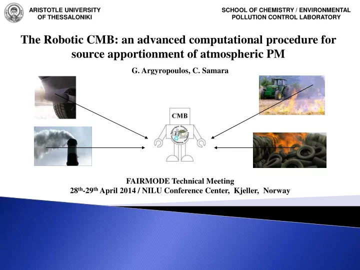
  1. ARISTOTLE UNIVERSITY SCHOOL OF CHEMISTRY / ENVIRONMENTAL OF THESSALONIKI POLLUTION CONTROL LABORATORY The Robotic CMB: an advanced computational procedure for source apportionment of atmospheric PM G. Argyropoulos, C. Samara FAIRMODE Technical Meeting 28 th -29 th April 2014 / NILU Conference Center, Kjeller, Norway

  2. ARISTOTLE UNIVERSITY SCHOOL OF CHEMISTRY / ENVIRONMENTAL OF THESSALONIKI POLLUTION CONTROL LABORATORY Introduction-Fundamental Concepts of CMB modeling Chemical Mass Balance (CMB) modeling is realized by solving an over determined system of linear equations which express ambient concentrations of chemical species measured at the receptor site as sums of contributions from individual sources: n C a S i ij j j 1 i = 1, 2, .., m j = 1, 2, …, n m > n Where C i is the mass concentration of chemical species i in ambient PM, α ij is the mass fraction of chemical species i in the PM emitted from source j, and S j is the contribution of source j to the total mass of ambient PM.

  3. ARISTOTLE UNIVERSITY SCHOOL OF CHEMISTRY / ENVIRONMENTAL OF THESSALONIKI POLLUTION CONTROL LABORATORY The main assumptions on which CMB models rely can be summarized as follows: • All the sources, contributing significantly to a receptor site, have been identified and have had their emissions chemically characterized. • Chemical species do not react with each other, i.e. they add linearly. • Compositions of source emissions remain constant during ambient and source sampling. • Source compositions are linearly independent of each other. • Measurement uncertainties are random, uncorrelated and normally distributed.

  4. ARISTOTLE UNIVERSITY SCHOOL OF CHEMISTRY / ENVIRONMENTAL OF THESSALONIKI POLLUTION CONTROL LABORATORY Least Squares (LS) Estimators of Source Contributions ( S j ) • Ordinary Least Squares (OLS) The OLS fitting method can estimate a set of probable values for the source contributions Sj , by minimizing the following likelihood function: System of Normal Equations 2 2 m n 2 T T C a S 0 A A S A C i ij j S i 1 j 1 j T 1 T S ( A A ) A C C a ... a S 1 1 11 1 n C ... S ... A ... ... ... Where S C a ... a n m m 1 mn and superscript T denotes the transpose matrix

  5. ARISTOTLE UNIVERSITY SCHOOL OF CHEMISTRY / ENVIRONMENTAL OF THESSALONIKI POLLUTION CONTROL LABORATORY • Ordinary Weighted Least Squares (OWLS) The OWLS fitting method can estimate a set of probable values for the source contributions ( S j ), by minimizing the following likelihood function, in which the heteroscedasticity of the receptor’s chemical data is reflected as well (Friedlander, 1973): 2 n C a S i ij j 2 m j 1 1 T T 2 S ( A W A ) A W C 0 … 2 S i 1 C j i 2 ... 0 C 1 And denotes the C i W ... ... ... Where typical error in the measurement of C i . 2 0 ... C m

  6. ARISTOTLE UNIVERSITY SCHOOL OF CHEMISTRY / ENVIRONMENTAL OF THESSALONIKI POLLUTION CONTROL LABORATORY • The Britt and Luecke Algorithm The Britt and Luecke algorithm consists of an iterative procedure that may estimate a set of probable values for the source contributions S j , in which all the measurement uncertainties are reflected, by minimizing the following likelihood function (Britt and Luecke, 1973;Watson et al., 1984): 2 n C a S 2 i ij j m m n a a j 1 ij ij 2 2 2 i 1 i 1 j 1 C a i ij Where the over bars indicate the “real” values of the mass fractions

  7. ARISTOTLE UNIVERSITY SCHOOL OF CHEMISTRY / ENVIRONMENTAL OF THESSALONIKI POLLUTION CONTROL LABORATORY Iteration Steps of the Britt and Luecke Algorithm • All the estimates for the source contributions S j are initially set equal to zero. • k ) -1 are determined The diagonal elements of the effective weighting matrix ( V e according to the following relationship: 1 n 1 2 k 2 2 k v S e , ii C j i ij j 1 Where superscript k indicates the iteration’s number.

  8. ARISTOTLE UNIVERSITY SCHOOL OF CHEMISTRY / ENVIRONMENTAL OF THESSALONIKI POLLUTION CONTROL LABORATORY • The new estimates for the “real” values of the mass fractions are calculated for each source profile ( j = 1,2, … , n ) by: 1 1 1 1 k 1 k k k k kT k k kT k k A A S V V I A A V A A V C AS j j j A e e e j Where V A j is one m x m diagonal matrix with elements on the diagonal and I is the m x m identity matrix. • Finally, the new estimates for the source contributions S j are calculated by: 1 1 1 k 1 k kT k k kT k k S S A V A A V C AS e e

  9. ARISTOTLE UNIVERSITY SCHOOL OF CHEMISTRY / ENVIRONMENTAL OF THESSALONIKI POLLUTION CONTROL LABORATORY • The Effective Variance Weighting Least Squares (EFWLS) The least squares fitting method of Britt and Luecke can be simplified substantially if the differences between the “true” values of the mass fractions and the measured ones are considered as negligible, allowing for the following likelihood function to be minimized (Watson et al., 1984): 2 n C a S i ij j m j 1 2 n 2 2 2 k i 1 S C j i ij j 1 This approximation (EFWLS) is currently the official method suggested by the Environmental Protection Agency of United States (US EPA) for CMB modeling.

  10. ARISTOTLE UNIVERSITY SCHOOL OF CHEMISTRY / ENVIRONMENTAL OF THESSALONIKI POLLUTION CONTROL LABORATORY Application of CMB models for the SA of ambient PM • Although CMB modeling is founded upon the “working hypothesis” that every source, which contributes significantly to the receptor site, has been identified, it is most often applied without any definite knowledge about the ones that actually do, since the identification of contributing sources may indeed be one of the major goals of a Source Apportionment (SA) study, under normal circumstances. • CMB modeling also requires that source compositions remain constant over the period of ambient and source sampling, which is, nonetheless, unlikely to occur. • There is virtually nothing to do too, in order to predict an occurrence of collinearity among the columns of the effectively weighted source profile matrix during run-time, in case that the algorithm of Britt and Luecke, or the EFWLS approximation has been adopted for the solution of the CMB problem.

  11. ARISTOTLE UNIVERSITY SCHOOL OF CHEMISTRY / ENVIRONMENTAL OF THESSALONIKI POLLUTION CONTROL LABORATORY • Due to those common violations of CMB assumptions, CMB modeling involves in practice first some test applications of the desired LS fitting method to over determined linear systems defined by different chemical species and/or source profiles, which have been all considered as equally probable for reflecting the true emissions at the receptor site, according to the personal judgment of the modeler. • According to the US EPA Protocol for Applying and Validating the CMB model (Watson, 2004), trial CMB tests should first be realized for an averaged ambient sample, in order to obtain the so-called “initial source contribution estimates”, i.e. to select a default combination of source profiles and fitting species for the ambient data.

  12. ARISTOTLE UNIVERSITY SCHOOL OF CHEMISTRY / ENVIRONMENTAL OF THESSALONIKI POLLUTION CONTROL LABORATORY • According to the same protocol, the initial source contribution estimates should then be optimized separately for each daily ambient sample, again by trial CMBs involving addition, depletion or substitution of source profiles, after taking into account additional factors, such as wind direction or the presumed temporal variation of sources such as biomass burnings. • The US EPA has also established a standard set of statistical performance measures for the evaluation of trial applications, which are given in the following table.

  13. ARISTOTLE UNIVERSITY SCHOOL OF CHEMISTRY / ENVIRONMENTAL OF THESSALONIKI POLLUTION CONTROL LABORATORY Diagnostic criteria of the US EPA CMB 8.2 model Performance measure(s) Target value(s) (US EPA) S j >0 2 2 R 1 0 . 8 m 1 2 k C i v e , ii i 1 2 2 4 red . m n n S j j 1 % mass = 100 100 % 20 % C mass E FracEst = n 1 S j Tstat 2 j var( S ) j k A S C i i │(Res/Uncer) i │ ≤2 (Res/Uncer) i 2 n 2 S C j i ij j 1 Overall Fitting Index 1 % mass 2 wf wf R wf wf FracEst 1 2 3 4 2 100 FitMeasure wf wf wf wf 1 2 3 4

  14. ARISTOTLE UNIVERSITY SCHOOL OF CHEMISTRY / ENVIRONMENTAL OF THESSALONIKI POLLUTION CONTROL LABORATORY Limitations of conventional CMB modeling • A major drawback of conventional CMB modeling arises from the fact that standard trial-and-error procedures are strongly subjected to the personal judgment of the modeler and his/her choices of fitting species/source profiles. • The trial CMBs of standard procedures are also limited to a total number far less than the ones that can possibly be defined by a typical set of input data, usually a few hundred or so. • The US EPA CMB 8.2 model, in particular, operating in Best Fit Mode, is capable of ranking, according to the Fit Measure index, a maximum of only 10 over determined linear systems, whose fitting species and source profiles must have been manually selected by the CMB modeler, using 10 pairs of species and profiles selection arrays that are provided for this purpose, by the model’s graphical user interface (Coulter, 2004).

Download Presentation
Download Policy: The content available on the website is offered to you 'AS IS' for your personal information and use only. It cannot be commercialized, licensed, or distributed on other websites without prior consent from the author. To download a presentation, simply click this link. If you encounter any difficulties during the download process, it's possible that the publisher has removed the file from their server.

Recommend


More recommend