The Language Modeling Problem We have some vocabulary, say V = { - PowerPoint PPT Presentation

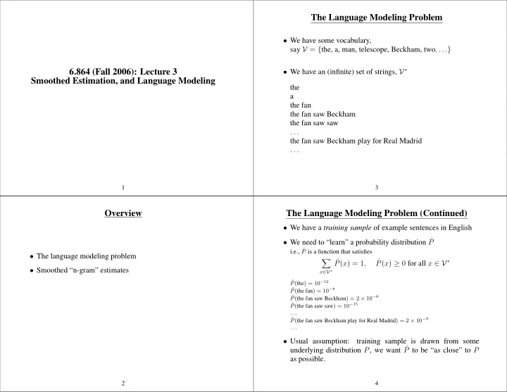
The Language Modeling Problem • We have some vocabulary, say V = { the, a, man, telescope, Beckham, two , . . . } • We have an (infinite) set of strings, V ∗ 6.864 (Fall 2006): Lecture 3 Smoothed Estimation, and Language Modeling the a the fan the fan saw Beckham the fan saw saw . . . the fan saw Beckham play for Real Madrid . . . 1 3 Overview The Language Modeling Problem (Continued) • We have a training sample of example sentences in English • We need to “learn” a probability distribution ˆ P i.e., ˆ P is a function that satisfies • The language modeling problem ˆ ˆ P ( x ) ≥ 0 for all x ∈ V ∗ � P ( x ) = 1 , • Smoothed “n-gram” estimates x ∈V ∗ ˆ P ( the ) = 10 − 12 ˆ P ( the fan ) = 10 − 8 P ( the fan saw Beckham ) = 2 × 10 − 8 ˆ ˆ P ( the fan saw saw ) = 10 − 15 . . . ˆ P ( the fan saw Beckham play for Real Madrid ) = 2 × 10 − 9 . . . • Usual assumption: training sample is drawn from some underlying distribution P , we want ˆ P to be “as close” to P as possible. 2 4

Why on earth would we want to do this?! Deriving a Trigram Probability Model Step 2: Make Markov independence assumptions: • Speech recognition was the original motivation. (Related problems are optical character recognition, handwriting P ( w 1 , w 2 , . . . , w n ) P ( w 1 | START ) = recognition.) × P ( w 2 | START , w 1 ) × P ( w 3 | w 1 , w 2 ) . . . • The estimation techniques developed for this problem will be × P ( w n | w n − 2 , w n − 1 ) VERY useful for other problems in NLP × P ( STOP | w n − 1 , w n ) General assumption: P ( w i | START , w 1 , w 2 , . . . , w i − 2 , w i − 1 ) = P ( w i | w i − 2 , w i − 1 ) For Example P ( the, dog, laughs ) = P ( the | START ) × P ( dog | START, the ) × P ( laughs | the, dog ) × P ( STOP | dog, laughs ) 5 7 The Trigram Estimation Problem Deriving a Trigram Probability Model Remaining estimation problem: Step 1: Expand using the chain rule: P ( w i | w i − 2 , w i − 1 ) P ( w 1 , w 2 , . . . , w n ) P ( w 1 | START ) = For example: × P ( w 2 | START , w 1 ) × P ( w 3 | START , w 1 , w 2 ) P ( laughs | the, dog ) × P ( w 4 | START , w 1 , w 2 , w 3 ) . . . × P ( w n | START , w 1 , w 2 , . . . , w n − 1 ) A natural estimate (the “maximum likelihood estimate”): × P ( STOP | START , w 1 , w 2 , . . . , w n − 1 , w n ) For Example P ML ( w i | w i − 2 , w i − 1 ) = Count ( w i , w i − 2 , w i − 1 ) Count ( w i − 2 , w i − 1 ) P ( the, dog, laughs ) P ( the | START ) = × P ( dog | START, the ) P ML ( laughs | the, dog ) = Count ( the, dog, laughs ) × P ( laughs | START, the, dog ) Count ( the, dog ) × P ( STOP | START, the, dog, laughs ) 6 8

Evaluating a Language Model Some History • We have some test data, n sentences • Shannon conducted experiments on entropy of English i.e., how good are people at the perplexity game? S 1 , S 2 , S 3 , . . . , S n C. Shannon. Prediction and entropy of printed • We could look at the probability under our model � n i =1 P ( S i ) . English. Bell Systems Technical Journal, 30:50–64, Or more conveniently, the log probability 1951. n n � � log P ( S i ) = log P ( S i ) i =1 i =1 • In fact the usual evaluation measure is perplexity n x = 1 Perplexity = 2 − x � log P ( S i ) where W i =1 and W is the total number of words in the test data. 9 11 Some Intuition about Perplexity Some History • Chomsky (in Syntactic Structures (1957)): • Say we have a vocabulary V , of size N = |V| Second, the notion “ grammatical” cannot be identified with and model that predicts “ meaningful”or “ significant”in any semantic sense. Sentences (1) and (2) are equally nonsensical, but any speaker of English P ( w ) = 1 will recognize that only the former is grammatical. N (1) Colorless green ideas sleep furiously. for all w ∈ V . (2) Furiously sleep ideas green colorless. . . . • Easy to calculate the perplexity in this case: . . . Third, the notion “ grammatical in English” cannot be identified in any way with the notion “ high order of statistical x = log 1 Perplexity = 2 − x approximation to English”. It is fair to assume that neither where N sentence (1) nor (2) (nor indeed any part of these sentences) has ⇒ ever occurred in an English discourse. Hence, in any statistical model for grammaticalness, these sentences will be ruled out Perplexity = N on identical grounds as equally ‘remote’ from English. Yet (1), though nonsensical, is grammatical, while (2) is not. . . . Perplexity is a measure of effective “branching factor” (my emphasis) 10 12

Sparse Data Problems Linear Interpolation A natural estimate (the “ maximum likelihood estimate”): • Take our estimate ˆ P ( w i | w i − 2 , w i − 1 ) to be P ML ( w i | w i − 2 , w i − 1 ) = Count ( w i − 2 , w i − 1 , w i ) ˆ P ( w i | w i − 2 , w i − 1 ) = λ 1 × P ML ( w i | w i − 2 , w i − 1 ) Count ( w i − 2 , w i − 1 ) + λ 2 × P ML ( w i | w i − 1 ) P ML ( laughs | the, dog ) = Count ( the, dog, laughs ) + λ 3 × P ML ( w i ) Count ( the, dog ) where λ 1 + λ 2 + λ 3 = 1 , and λ i ≥ 0 for all i . Say our vocabulary size is N = |V| , then there are N 3 parameters in the model. 20 , 000 3 = 8 × 10 12 parameters e.g., N = 20 , 000 ⇒ 13 15 The Bias-Variance Trade-Off • Our estimate correctly defines a distribution: • (Unsmoothed) trigram estimate w ∈V ˆ � P ( w | w i − 2 , w i − 1 ) P ML ( w i | w i − 2 , w i − 1 ) = Count ( w i − 2 , w i − 1 , w i ) = � w ∈V [ λ 1 × P ML ( w | w i − 2 , w i − 1 ) + λ 2 × P ML ( w | w i − 1 ) + λ 3 × P ML ( w )] Count ( w i − 2 , w i − 1 ) � � � = λ 1 w P ML ( w | w i − 2 , w i − 1 ) + λ 2 w P ML ( w | w i − 1 ) + λ 3 w P ML ( w ) • (Unsmoothed) bigram estimate = λ 1 + λ 2 + λ 3 P ML ( w i | w i − 1 ) = Count ( w i − 1 , w i ) = 1 Count ( w i − 1 ) (Can show also that ˆ P ( w | w i − 2 , w i − 1 ) ≥ 0 for all w ∈ V ) • (Unsmoothed) unigram estimate P ML ( w i ) = Count ( w i ) Count () How close are these different estimates to the “true” probability P ( w i | w i − 2 , w i − 1 ) ? 14 16

How to estimate the λ values? Allowing the λ ’s to vary • Hold out part of training set as “validation” data • Take a function Φ that partitions histories e.g., • Define Count 2 ( w 1 , w 2 , w 3 ) to be the number of times the 1 If Count ( w i − 1 , w i − 2 ) = 0   trigram ( w 1 , w 2 , w 3 ) is seen in validation set  2 If 1 ≤ Count ( w i − 1 , w i − 2 ) ≤ 2   Φ( w i − 2 , w i − 1 ) = 3 If 3 ≤ Count ( w i − 1 , w i − 2 ) ≤ 5    4 • Choose λ 1 , λ 2 , λ 3 to maximize: Otherwise  Count 2 ( w 1 , w 2 , w 3 ) log ˆ � L ( λ 1 , λ 2 , λ 3 ) = P ( w 3 | w 1 , w 2 ) • Introduce a dependence of the λ ’s on the partition: w 1 ,w 2 ,w 3 ∈V ˆ λ Φ( w i − 2 ,w i − 1 ) P ( w i | w i − 2 , w i − 1 ) = × P ML ( w i | w i − 2 , w i − 1 ) 1 such that λ 1 + λ 2 + λ 3 = 1 , and λ i ≥ 0 for all i , and where + λ Φ( w i − 2 ,w i − 1 ) × P ML ( w i | w i − 1 ) 2 ˆ P ( w i | w i − 2 , w i − 1 ) = λ 1 × P ML ( w i | w i − 2 , w i − 1 ) + λ Φ( w i − 2 ,w i − 1 ) × P ML ( w i ) 3 + λ 2 × P ML ( w i | w i − 1 ) where λ Φ( w i − 2 ,w i − 1 ) + λ Φ( w i − 2 ,w i − 1 ) + λ Φ( w i − 2 ,w i − 1 ) + λ 3 × P ML ( w i ) = 1 , and 1 2 3 λ Φ( w i − 2 ,w i − 1 ) ≥ 0 for all i . i 17 19 An Iterative Method • Our estimate correctly defines a distribution: Initialization: Pick arbitrary/random values for λ 1 , λ 2 , λ 3 . w ∈V ˆ � P ( w | w i − 2 , w i − 1 ) Step 1: Calculate the following quantities: Φ( w i − 2 ,w i − 1 ) Count 2 ( w 1 , w 2 , w 3 ) λ 1 P ML ( w 3 | w 1 , w 2 ) = � w ∈V [ λ × P ML ( w | w i − 2 , w i − 1 ) � = 1 c 1 Φ( w i − 2 ,w i − 1 ) λ 1 P ML ( w 3 | w 1 , w 2 ) + λ 2 P ML ( w 3 | w 2 ) + λ 3 P ML ( w 3 ) + λ × P ML ( w | w i − 1 ) 2 w 1 ,w 2 ,w 3 ∈V Φ( w i − 2 ,w i − 1 ) + λ × P ML ( w )] 3 Count 2 ( w 1 , w 2 , w 3 ) λ 2 P ML ( w 3 | w 2 ) � c 2 = Φ( w i − 2 ,w i − 1 ) λ 1 P ML ( w 3 | w 1 , w 2 ) + λ 2 P ML ( w 3 | w 2 ) + λ 3 P ML ( w 3 ) = λ � w P ML ( w | w i − 2 , w i − 1 ) 1 w 1 ,w 2 ,w 3 ∈V Φ( w i − 2 ,w i − 1 ) + λ � w P ML ( w | w i − 1 ) 2 Φ( w i − 2 ,w i − 1 ) Count 2 ( w 1 , w 2 , w 3 ) λ 3 P ML ( w 3 ) + λ � w P ML ( w ) � = c 3 3 λ 1 P ML ( w 3 | w 1 , w 2 ) + λ 2 P ML ( w 3 | w 2 ) + λ 3 P ML ( w 3 ) w 1 ,w 2 ,w 3 ∈V Φ( w i − 2 ,w i − 1 ) Φ( w i − 2 ,w i − 1 ) Φ( w i − 2 ,w i − 1 ) = λ + λ + λ 1 2 3 Step 2: Re-estimate λ i ’s as = 1 c 1 c 2 c 3 λ 1 = , λ 2 = , λ 3 = c 1 + c 2 + c 3 c 1 + c 2 + c 3 c 1 + c 2 + c 3 Step 3: If λ i ’s have not converged, go to Step 1 . 18 20