The densest subgraph of sparse random graphs Justin Salez (Universit - - PowerPoint PPT Presentation

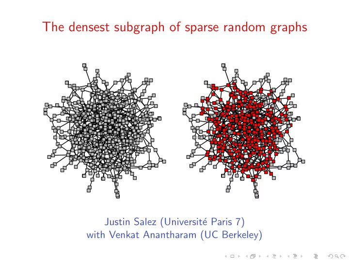
The densest subgraph of sparse random graphs

Justin Salez (Universit´ e Paris 7) with Venkat Anantharam (UC Berkeley)

The objective method (Aldous-Steele, 2004)

The objective method (Aldous-Steele, 2004)

◮ Context: given a large interacting system (graph), one is

interested in a macroscopic quantity which depends on the microscopic contribution of each particle (vertices).

The objective method (Aldous-Steele, 2004)

◮ Context: given a large interacting system (graph), one is

interested in a macroscopic quantity which depends on the microscopic contribution of each particle (vertices).

◮ Key assumption: no long-range interactions, i.e. the

microscopic contribution of each particle is essentially insensitive to remote perturbations of the system.

The objective method (Aldous-Steele, 2004)

◮ Context: given a large interacting system (graph), one is

interested in a macroscopic quantity which depends on the microscopic contribution of each particle (vertices).

◮ Key assumption: no long-range interactions, i.e. the

microscopic contribution of each particle is essentially insensitive to remote perturbations of the system.

◮ Expected consequences:

The objective method (Aldous-Steele, 2004)

◮ Context: given a large interacting system (graph), one is

interested in a macroscopic quantity which depends on the microscopic contribution of each particle (vertices).

◮ Key assumption: no long-range interactions, i.e. the

microscopic contribution of each particle is essentially insensitive to remote perturbations of the system.

◮ Expected consequences:

• 1. efficient approximability by local distributed algorithms;

The objective method (Aldous-Steele, 2004)

◮ Context: given a large interacting system (graph), one is

interested in a macroscopic quantity which depends on the microscopic contribution of each particle (vertices).

◮ Key assumption: no long-range interactions, i.e. the

microscopic contribution of each particle is essentially insensitive to remote perturbations of the system.

◮ Expected consequences:

• 1. efficient approximability by local distributed algorithms;
• 2. existence of an infinite-volume limit.

The objective method (Aldous-Steele, 2004)

◮ Context: given a large interacting system (graph), one is

interested in a macroscopic quantity which depends on the microscopic contribution of each particle (vertices).

◮ Key assumption: no long-range interactions, i.e. the

microscopic contribution of each particle is essentially insensitive to remote perturbations of the system.

◮ Expected consequences:

• 1. efficient approximability by local distributed algorithms;
• 2. existence of an infinite-volume limit.

◮ Idea: formalize that via local weak convergence, and use this

framework to replace the asymptotic study of large graphs by the direct analysis of their infinite-volume limits.

Local convergence around a fixed root

Local convergence around a fixed root

(G, o) : countable, locally finite, connected rooted graph

Local convergence around a fixed root

(G, o) : countable, locally finite, connected rooted graph [G, o]R : ball of radius R around o in G

Local convergence around a fixed root

(G, o) : countable, locally finite, connected rooted graph [G, o]R : ball of radius R around o in G

R

Local convergence around a fixed root

(G, o) : countable, locally finite, connected rooted graph [G, o]R : ball of radius R around o in G

R

(Gn, on) − − − →

n→∞ (G, o)

Local convergence around a fixed root

(G, o) : countable, locally finite, connected rooted graph [G, o]R : ball of radius R around o in G

R

(Gn, on) − − − →

n→∞ (G, o) if for each fixed R, there is nR ∈ N such that

n ≥ nR = ⇒ [Gn, on]R ≡ [G, o]R

Local weak convergence (Benjamini-Schramm, 2001)

G⋆ = {locally finite connected rooted graphs}.

Local weak convergence (Benjamini-Schramm, 2001)

G⋆ = {locally finite connected rooted graphs}. G = (V , E) : finite unrooted, possibly disconnected graph.

Local weak convergence (Benjamini-Schramm, 2001)

G⋆ = {locally finite connected rooted graphs}. G = (V , E) : finite unrooted, possibly disconnected graph. Consider the law on G⋆ obtained by choosing a root o ∈ V uniformly at random, and restricting to its connected component:

Local weak convergence (Benjamini-Schramm, 2001)

G⋆ = {locally finite connected rooted graphs}. G = (V , E) : finite unrooted, possibly disconnected graph. Consider the law on G⋆ obtained by choosing a root o ∈ V uniformly at random, and restricting to its connected component: LG := 1 |V |

• ∈V

δ[G,o].

Local weak convergence (Benjamini-Schramm, 2001)

G⋆ = {locally finite connected rooted graphs}. G = (V , E) : finite unrooted, possibly disconnected graph. Consider the law on G⋆ obtained by choosing a root o ∈ V uniformly at random, and restricting to its connected component: LG := 1 |V |

• ∈V

δ[G,o]. LG is an element of P(G⋆) := {probability measures on G⋆}.

Local weak convergence (Benjamini-Schramm, 2001)

G⋆ = {locally finite connected rooted graphs}. G = (V , E) : finite unrooted, possibly disconnected graph. Consider the law on G⋆ obtained by choosing a root o ∈ V uniformly at random, and restricting to its connected component: LG := 1 |V |

• ∈V

δ[G,o]. LG is an element of P(G⋆) := {probability measures on G⋆}. {Gn}n≥1 : sequence of finite graphs.

Local weak convergence (Benjamini-Schramm, 2001)

G⋆ = {locally finite connected rooted graphs}. G = (V , E) : finite unrooted, possibly disconnected graph. Consider the law on G⋆ obtained by choosing a root o ∈ V uniformly at random, and restricting to its connected component: LG := 1 |V |

• ∈V

δ[G,o]. LG is an element of P(G⋆) := {probability measures on G⋆}. {Gn}n≥1 : sequence of finite graphs. If {LGn}n≥1 admits a weak limit L ∈ P(G⋆), then call L the local weak limit of {Gn}n≥1.

Local weak convergence (Benjamini-Schramm, 2001)

G⋆ = {locally finite connected rooted graphs}. G = (V , E) : finite unrooted, possibly disconnected graph. Consider the law on G⋆ obtained by choosing a root o ∈ V uniformly at random, and restricting to its connected component: LG := 1 |V |

• ∈V

δ[G,o]. LG is an element of P(G⋆) := {probability measures on G⋆}. {Gn}n≥1 : sequence of finite graphs. If {LGn}n≥1 admits a weak limit L ∈ P(G⋆), then call L the local weak limit of {Gn}n≥1. ◮ L describes the local geometry of Gn around a random node

Examples of local weak limits

Examples of local weak limits

Note: graphs must be sparse, i.e. |E| ≍ |V |

Examples of local weak limits

Note: graphs must be sparse, i.e. |E| ≍ |V |

◮ Gn = box of size n × . . . × n in Zd

Examples of local weak limits

Note: graphs must be sparse, i.e. |E| ≍ |V |

◮ Gn = box of size n × . . . × n in Zd

L = dirac at (Zd, 0)

Examples of local weak limits

Note: graphs must be sparse, i.e. |E| ≍ |V |

◮ Gn = box of size n × . . . × n in Zd

L = dirac at (Zd, 0)

◮ Gn = random d−regular graph on n nodes

Examples of local weak limits

Note: graphs must be sparse, i.e. |E| ≍ |V |

◮ Gn = box of size n × . . . × n in Zd

L = dirac at (Zd, 0)

◮ Gn = random d−regular graph on n nodes

L = dirac at the d−regular infinite rooted tree

Examples of local weak limits

Note: graphs must be sparse, i.e. |E| ≍ |V |

◮ Gn = box of size n × . . . × n in Zd

L = dirac at (Zd, 0)

◮ Gn = random d−regular graph on n nodes

L = dirac at the d−regular infinite rooted tree

◮ Gn = Erd˝

• s-R´

enyi graph with pn = c

n on n nodes

Examples of local weak limits

Note: graphs must be sparse, i.e. |E| ≍ |V |

◮ Gn = box of size n × . . . × n in Zd

L = dirac at (Zd, 0)

◮ Gn = random d−regular graph on n nodes

L = dirac at the d−regular infinite rooted tree

◮ Gn = Erd˝

• s-R´

enyi graph with pn = c

n on n nodes

L = law of a Galton-Watson tree with degree Poisson(c)

Examples of local weak limits

Note: graphs must be sparse, i.e. |E| ≍ |V |

◮ Gn = box of size n × . . . × n in Zd

L = dirac at (Zd, 0)

◮ Gn = random d−regular graph on n nodes

L = dirac at the d−regular infinite rooted tree

◮ Gn = Erd˝

• s-R´

enyi graph with pn = c

n on n nodes

L = law of a Galton-Watson tree with degree Poisson(c)

◮ Gn = random graph with degree distribution π on n nodes

Examples of local weak limits

Note: graphs must be sparse, i.e. |E| ≍ |V |

◮ Gn = box of size n × . . . × n in Zd

L = dirac at (Zd, 0)

◮ Gn = random d−regular graph on n nodes

L = dirac at the d−regular infinite rooted tree

◮ Gn = Erd˝

• s-R´

enyi graph with pn = c

n on n nodes

L = law of a Galton-Watson tree with degree Poisson(c)

◮ Gn = random graph with degree distribution π on n nodes

L = law of a Galton-Watson tree with degree distribution π

Examples of local weak limits

Note: graphs must be sparse, i.e. |E| ≍ |V |

◮ Gn = box of size n × . . . × n in Zd

L = dirac at (Zd, 0)

◮ Gn = random d−regular graph on n nodes

L = dirac at the d−regular infinite rooted tree

◮ Gn = Erd˝

• s-R´

enyi graph with pn = c

n on n nodes

L = law of a Galton-Watson tree with degree Poisson(c)

◮ Gn = random graph with degree distribution π on n nodes

L = law of a Galton-Watson tree with degree distribution π

◮ Gn = uniform random tree on n nodes

Examples of local weak limits

Note: graphs must be sparse, i.e. |E| ≍ |V |

◮ Gn = box of size n × . . . × n in Zd

L = dirac at (Zd, 0)

◮ Gn = random d−regular graph on n nodes

L = dirac at the d−regular infinite rooted tree

◮ Gn = Erd˝

• s-R´

enyi graph with pn = c

n on n nodes

L = law of a Galton-Watson tree with degree Poisson(c)

◮ Gn = random graph with degree distribution π on n nodes

L = law of a Galton-Watson tree with degree distribution π

◮ Gn = uniform random tree on n nodes

L = Infinite Skeleton Tree (Grimmett, 1980)

Examples of local weak limits

Note: graphs must be sparse, i.e. |E| ≍ |V |

◮ Gn = box of size n × . . . × n in Zd

L = dirac at (Zd, 0)

◮ Gn = random d−regular graph on n nodes

L = dirac at the d−regular infinite rooted tree

◮ Gn = Erd˝

• s-R´

enyi graph with pn = c

n on n nodes

L = law of a Galton-Watson tree with degree Poisson(c)

◮ Gn = random graph with degree distribution π on n nodes

L = law of a Galton-Watson tree with degree distribution π

◮ Gn = uniform random tree on n nodes

L = Infinite Skeleton Tree (Grimmett, 1980)

◮ Gn = preferential attachment graph on n nodes

Examples of local weak limits

Note: graphs must be sparse, i.e. |E| ≍ |V |

◮ Gn = box of size n × . . . × n in Zd

L = dirac at (Zd, 0)

◮ Gn = random d−regular graph on n nodes

L = dirac at the d−regular infinite rooted tree

◮ Gn = Erd˝

• s-R´

enyi graph with pn = c

n on n nodes

L = law of a Galton-Watson tree with degree Poisson(c)

◮ Gn = random graph with degree distribution π on n nodes

L = law of a Galton-Watson tree with degree distribution π

◮ Gn = uniform random tree on n nodes

L = Infinite Skeleton Tree (Grimmett, 1980)

◮ Gn = preferential attachment graph on n nodes

L = Polya-point graph (Berger-Borgs-Chayes-Sabery, 2009)

An illustration: the nullity of large graphs

An illustration: the nullity of large graphs

µG({0}) = dim ker(AG)

|V |

.

An illustration: the nullity of large graphs

µG({0}) = dim ker(AG)

|V |

. Asymptotics when G is large ?

An illustration: the nullity of large graphs

µG({0}) = dim ker(AG)

|V |

. Asymptotics when G is large ? Conjecture (Bauer-Golinelli 2001). For Gn : Erd˝

• s-R´

enyi

• n, c

n

• ,

µGn({0}) − − − →

n→∞

λ∗ + e−cλ∗ + cλ∗e−cλ∗ − 1, where λ∗ ∈ [0, 1] is the smallest root of λ = e−ce−cλ.

An illustration: the nullity of large graphs

µG({0}) = dim ker(AG)

|V |

. Asymptotics when G is large ? Conjecture (Bauer-Golinelli 2001). For Gn : Erd˝

• s-R´

enyi

• n, c

n

• ,

µGn({0}) − − − →

n→∞

λ∗ + e−cλ∗ + cλ∗e−cλ∗ − 1, where λ∗ ∈ [0, 1] is the smallest root of λ = e−ce−cλ. Theorem (Bordenave-Lelarge-S., 2011)

An illustration: the nullity of large graphs

µG({0}) = dim ker(AG)

|V |

. Asymptotics when G is large ? Conjecture (Bauer-Golinelli 2001). For Gn : Erd˝

• s-R´

enyi

• n, c

n

• ,

µGn({0}) − − − →

n→∞

λ∗ + e−cλ∗ + cλ∗e−cλ∗ − 1, where λ∗ ∈ [0, 1] is the smallest root of λ = e−ce−cλ. Theorem (Bordenave-Lelarge-S., 2011)

• 1. Gn → L =

⇒ µGn({0}) → µL({0}).

An illustration: the nullity of large graphs

µG({0}) = dim ker(AG)

|V |

. Asymptotics when G is large ? Conjecture (Bauer-Golinelli 2001). For Gn : Erd˝

• s-R´

enyi

• n, c

n

• ,

µGn({0}) − − − →

n→∞

λ∗ + e−cλ∗ + cλ∗e−cλ∗ − 1, where λ∗ ∈ [0, 1] is the smallest root of λ = e−ce−cλ. Theorem (Bordenave-Lelarge-S., 2011)

• 1. Gn → L =

⇒ µGn({0}) → µL({0}).

• 2. When L = Galton-Watson(π),

µL({0}) = min

λ=λ∗∗

• f ′(1)λλ∗ + f (1 − λ) + f (1 − λ∗) − 1
• ,

where f (z) =

n πnzn and λ∗ = f ′(1 − λ)/f ′(1).

Continuity with respect to local weak convergence

Continuity with respect to local weak convergence

◮ In the sparse regime, many important graph parameters Φ are

essentially determined by the local geometry only.

Continuity with respect to local weak convergence

◮ In the sparse regime, many important graph parameters Φ are

essentially determined by the local geometry only.

◮ This can be rigorously formalized by a continuity theorem:

Gn

loc.

− − − →

n→∞ L

= ⇒ Φ(Gn) − − − →

n→∞ Φ(L)

Continuity with respect to local weak convergence

◮ In the sparse regime, many important graph parameters Φ are

essentially determined by the local geometry only.

◮ This can be rigorously formalized by a continuity theorem:

Gn

loc.

− − − →

n→∞ L

= ⇒ Φ(Gn) − − − →

n→∞ Φ(L) ◮ Algorithmic implication: Φ is efficiently approximable via

local distributed algorithms, independently of network size.

Continuity with respect to local weak convergence

◮ In the sparse regime, many important graph parameters Φ are

essentially determined by the local geometry only.

◮ This can be rigorously formalized by a continuity theorem:

Gn

loc.

− − − →

n→∞ L

= ⇒ Φ(Gn) − − − →

n→∞ Φ(L) ◮ Algorithmic implication: Φ is efficiently approximable via

local distributed algorithms, independently of network size.

◮ Analytic implication: Φ admits a limit along most sparse

graph sequences. The distributional self-similarity of L may even allow for an explicit determination of Φ(L).

Continuity with respect to local weak convergence

◮ In the sparse regime, many important graph parameters Φ are

essentially determined by the local geometry only.

◮ This can be rigorously formalized by a continuity theorem:

Gn

loc.

− − − →

n→∞ L

= ⇒ Φ(Gn) − − − →

n→∞ Φ(L) ◮ Algorithmic implication: Φ is efficiently approximable via

local distributed algorithms, independently of network size.

◮ Analytic implication: Φ admits a limit along most sparse

graph sequences. The distributional self-similarity of L may even allow for an explicit determination of Φ(L).

◮ Examples:

Continuity with respect to local weak convergence

◮ In the sparse regime, many important graph parameters Φ are

essentially determined by the local geometry only.

◮ This can be rigorously formalized by a continuity theorem:

Gn

loc.

− − − →

n→∞ L

= ⇒ Φ(Gn) − − − →

n→∞ Φ(L) ◮ Algorithmic implication: Φ is efficiently approximable via

local distributed algorithms, independently of network size.

◮ Analytic implication: Φ admits a limit along most sparse

graph sequences. The distributional self-similarity of L may even allow for an explicit determination of Φ(L).

◮ Examples: number of spanning trees (Lyons, 2005),

Continuity with respect to local weak convergence

◮ In the sparse regime, many important graph parameters Φ are

essentially determined by the local geometry only.

◮ This can be rigorously formalized by a continuity theorem:

Gn

loc.

− − − →

n→∞ L

= ⇒ Φ(Gn) − − − →

n→∞ Φ(L) ◮ Algorithmic implication: Φ is efficiently approximable via

local distributed algorithms, independently of network size.

◮ Analytic implication: Φ admits a limit along most sparse

graph sequences. The distributional self-similarity of L may even allow for an explicit determination of Φ(L).

◮ Examples: number of spanning trees (Lyons, 2005), spectrum

and rank (Bordenave-Lelarge-S, 2011),

Continuity with respect to local weak convergence

◮ In the sparse regime, many important graph parameters Φ are

essentially determined by the local geometry only.

◮ This can be rigorously formalized by a continuity theorem:

Gn

loc.

− − − →

n→∞ L

= ⇒ Φ(Gn) − − − →

n→∞ Φ(L) ◮ Algorithmic implication: Φ is efficiently approximable via

local distributed algorithms, independently of network size.

◮ Analytic implication: Φ admits a limit along most sparse

graph sequences. The distributional self-similarity of L may even allow for an explicit determination of Φ(L).

◮ Examples: number of spanning trees (Lyons, 2005), spectrum

and rank (Bordenave-Lelarge-S, 2011), matching polynomial (idem, 2013),

Continuity with respect to local weak convergence

◮ In the sparse regime, many important graph parameters Φ are

essentially determined by the local geometry only.

◮ This can be rigorously formalized by a continuity theorem:

Gn

loc.

− − − →

n→∞ L

= ⇒ Φ(Gn) − − − →

n→∞ Φ(L) ◮ Algorithmic implication: Φ is efficiently approximable via

local distributed algorithms, independently of network size.

◮ Analytic implication: Φ admits a limit along most sparse

graph sequences. The distributional self-similarity of L may even allow for an explicit determination of Φ(L).

◮ Examples: number of spanning trees (Lyons, 2005), spectrum

and rank (Bordenave-Lelarge-S, 2011), matching polynomial (idem, 2013), Ising models (Dembo-Montanari-Sun, 2013)...

The densest subgraph problem

The densest subgraph problem

Fix a finite graph G = (V , E)

The densest subgraph problem

Fix a finite graph G = (V , E) Densest subgraph : H⋆ = argmax

• |E(H)|

|H| : H ⊆ V

The densest subgraph problem

Fix a finite graph G = (V , E) Densest subgraph : H⋆ = argmax

• |E(H)|

|H| : H ⊆ V

• Maximum subgraph density : ̺⋆ = max
• |E(H)|

|H| : H ⊆ V

The densest subgraph problem

Fix a finite graph G = (V , E) Densest subgraph : H⋆ = argmax

• |E(H)|

|H| : H ⊆ V

• Maximum subgraph density : ̺⋆ = max
• |E(H)|

|H| : H ⊆ V

• = 17

10

The densest subgraph problem on large sparse graphs

The densest subgraph problem on large sparse graphs

The densest subgraph problem on large sparse graphs

Load balancing

Load balancing

An allocation on G is a function θ: E → [0, 1] satisfying θ(i, j) + θ(j, i) = 1

Load balancing

An allocation on G is a function θ: E → [0, 1] satisfying θ(i, j) + θ(j, i) = 1 The induced load at i ∈ V is ∂θ(i) =

• j∼i

θ(j, i)

Load balancing

An allocation on G is a function θ: E → [0, 1] satisfying θ(i, j) + θ(j, i) = 1 The induced load at i ∈ V is ∂θ(i) =

• j∼i

θ(j, i) The allocation is balanced if for each (i, j) ∈ E ∂θ(i) < ∂θ(j) = ⇒ θ(i, j) = 0

From local to global optimality

From local to global optimality

• Claim. For an allocation θ, the following are equivalent:

From local to global optimality

• Claim. For an allocation θ, the following are equivalent:
• 1. θ is balanced

From local to global optimality

• Claim. For an allocation θ, the following are equivalent:
• 1. θ is balanced
• 2. θ minimizes

i (∂θ(i))2.

From local to global optimality

• Claim. For an allocation θ, the following are equivalent:
• 1. θ is balanced
• 2. θ minimizes

i (∂θ(i))2.

• 3. θ minimizes

i f (∂θ(i)) for any convex function f : R → R.

From local to global optimality

• Claim. For an allocation θ, the following are equivalent:
• 1. θ is balanced
• 2. θ minimizes

i (∂θ(i))2.

• 3. θ minimizes

i f (∂θ(i)) for any convex function f : R → R.

Corollary 1. Balanced allocations always exist.

From local to global optimality

• Claim. For an allocation θ, the following are equivalent:
• 1. θ is balanced
• 2. θ minimizes

i (∂θ(i))2.

• 3. θ minimizes

i f (∂θ(i)) for any convex function f : R → R.

Corollary 1. Balanced allocations always exist. Corollary 2. They all induce the same loads ∂θ: V → [0, ∞).

From local to global optimality

• Claim. For an allocation θ, the following are equivalent:
• 1. θ is balanced
• 2. θ minimizes

i (∂θ(i))2.

• 3. θ minimizes

i f (∂θ(i)) for any convex function f : R → R.

Corollary 1. Balanced allocations always exist. Corollary 2. They all induce the same loads ∂θ: V → [0, ∞). Corollary 3. Balanced loads solve the densest subgraph problem:

From local to global optimality

• Claim. For an allocation θ, the following are equivalent:
• 1. θ is balanced
• 2. θ minimizes

i (∂θ(i))2.

• 3. θ minimizes

i f (∂θ(i)) for any convex function f : R → R.

Corollary 1. Balanced allocations always exist. Corollary 2. They all induce the same loads ∂θ: V → [0, ∞). Corollary 3. Balanced loads solve the densest subgraph problem: max

i∈V ∂θ(i) = ̺⋆

and argmax

i∈V

∂θ(i) = H⋆

Example

Example

3 7 2 2 3 4 8 8 6 7 5 5 5 5 5 5 8 2 8 7 3 2 2 8 5 5 9 3 4 7 6 7 3 1 10 10 10 10 10 10 10 10 10 10 5 5 5 5 8 9 10 10 10 5 5 5 5 10 5 5 5 5 10 8 2 2 9 1 5 5 1 10

Example

1.5 1.5 1.5 1.5 1.5 1.5 1.5 1.5 1 1 1 1 1.7 1.7 1.7 1.7 1.7 1.7 1.7 1.7 1.7 1.7 1.6 1.6 1.6 1.6 1.6 1.5 1.5

Example

1.5 1.5 1.5 1.5 1.5 1.5 1.5 1.5 1 1 1 1 1.7 1.7 1.7 1.7 1.7 1.7 1.7 1.7 1.7 1.7 1.6 1.6 1.6 1.6 1.6 1.5 1.5

How do those ‘densities” look on a large sparse graph ?

How do those ‘densities” look on a large sparse graph ?

How do those ‘densities” look on a large sparse graph ?

Density profile of a random graph with average degree 3

Density profile of a random graph with average degree 3

|V | = 100

Density profile of a random graph with average degree 3

|V | = 100 |V | = 10000

Density profile of a random graph with average degree 4

Density profile of a random graph with average degree 4

|V | = 100

Density profile of a random graph with average degree 4

|V | = 100 |V | = 10000

The conjecture (Hajek, 1990)

The conjecture (Hajek, 1990)

∂Θ(G, o) : load induced at o by any balanced allocation on G.

The conjecture (Hajek, 1990)

∂Θ(G, o) : load induced at o by any balanced allocation on G. Define the density profile of G = (V , E) as ΛG = 1 |V |

• ∈V

δ∂Θ(G,o) ∈ P(R).

The conjecture (Hajek, 1990)

∂Θ(G, o) : load induced at o by any balanced allocation on G. Define the density profile of G = (V , E) as ΛG = 1 |V |

• ∈V

δ∂Θ(G,o) ∈ P(R). Conjecture: Gn Erd˝

• s-R´

enyi

• n, c

n

• ; c fixed, n → ∞

The conjecture (Hajek, 1990)

∂Θ(G, o) : load induced at o by any balanced allocation on G. Define the density profile of G = (V , E) as ΛG = 1 |V |

• ∈V

δ∂Θ(G,o) ∈ P(R). Conjecture: Gn Erd˝

• s-R´

enyi

• n, c

n

• ; c fixed, n → ∞
• 1. ΛGn concentrates around a deterministic Λ ∈ P(R)

The conjecture (Hajek, 1990)

∂Θ(G, o) : load induced at o by any balanced allocation on G. Define the density profile of G = (V , E) as ΛG = 1 |V |

• ∈V

δ∂Θ(G,o) ∈ P(R). Conjecture: Gn Erd˝

• s-R´

enyi

• n, c

n

• ; c fixed, n → ∞
• 1. ΛGn concentrates around a deterministic Λ ∈ P(R)
• 2. ̺⋆(Gn)

P

− − − →

n→∞ sup{t ∈ R: Λ(t, +∞) > 0}

Result 1 : the density profile of sparse graphs

Result 1 : the density profile of sparse graphs

• Theorem. Assume that L [deg(G, o)] < ∞.

Result 1 : the density profile of sparse graphs

• Theorem. Assume that L [deg(G, o)] < ∞. Then,

Gn

loc.

− − − →

n→∞ L

= ⇒ ΛGn

P(R)

− − − →

n→∞ ΛL

Result 1 : the density profile of sparse graphs

• Theorem. Assume that L [deg(G, o)] < ∞. Then,

Gn

loc.

− − − →

n→∞ L

= ⇒ ΛGn

P(R)

− − − →

n→∞ ΛL

where ΛL is the solution to a certain optimization problem on L.

Result 1 : the density profile of sparse graphs

• Theorem. Assume that L [deg(G, o)] < ∞. Then,

Gn

loc.

− − − →

n→∞ L

= ⇒ ΛGn

P(R)

− − − →

n→∞ ΛL

where ΛL is the solution to a certain optimization problem on L. Specifically, the excess function Φ: t →

• R(x − t)+ΛL(dx)

Result 1 : the density profile of sparse graphs

• Theorem. Assume that L [deg(G, o)] < ∞. Then,

Gn

loc.

− − − →

n→∞ L

= ⇒ ΛGn

P(R)

− − − →

n→∞ ΛL

where ΛL is the solution to a certain optimization problem on L. Specifically, the excess function Φ: t →

• R(x − t)+ΛL(dx) solves

Φ(t) = max

f : G⋆→[0,1]

• 1

2L

• i∼o

f (G, i) ∧ f (G, o)

• − tL[f (G, o)]

Result 2 : maximum subgraph density of sparse graphs

Result 2 : maximum subgraph density of sparse graphs

Extend the definition of ̺⋆ to local weak limits by ̺⋆(L) := sup ess ΛL = sup{t : Φ(t) > 0}

Result 2 : maximum subgraph density of sparse graphs

Extend the definition of ̺⋆ to local weak limits by ̺⋆(L) := sup ess ΛL = sup{t : Φ(t) > 0} In light of previous result, one expects a continuity principle :

Result 2 : maximum subgraph density of sparse graphs

Extend the definition of ̺⋆ to local weak limits by ̺⋆(L) := sup ess ΛL = sup{t : Φ(t) > 0} In light of previous result, one expects a continuity principle : Gn

loc.

− − − →

n→∞ L

= ⇒ ̺⋆(Gn) − − − →

n→∞ ̺⋆(L)

Result 2 : maximum subgraph density of sparse graphs

Extend the definition of ̺⋆ to local weak limits by ̺⋆(L) := sup ess ΛL = sup{t : Φ(t) > 0} In light of previous result, one expects a continuity principle : Gn

loc.

− − − →

n→∞ L

= ⇒ ̺⋆(Gn) − − − →

n→∞ ̺⋆(L)

Counter-example:

Result 2 : maximum subgraph density of sparse graphs

Extend the definition of ̺⋆ to local weak limits by ̺⋆(L) := sup ess ΛL = sup{t : Φ(t) > 0} In light of previous result, one expects a continuity principle : Gn

loc.

− − − →

n→∞ L

= ⇒ ̺⋆(Gn) − − − →

n→∞ ̺⋆(L)

Counter-example: adding a large but fixed clique to Gn will arbitrarily boost ̺⋆(Gn) without affecting convergence Gn → L.

Result 2 : maximum subgraph density of sparse graphs

Extend the definition of ̺⋆ to local weak limits by ̺⋆(L) := sup ess ΛL = sup{t : Φ(t) > 0} In light of previous result, one expects a continuity principle : Gn

loc.

− − − →

n→∞ L

= ⇒ ̺⋆(Gn) − − − →

n→∞ ̺⋆(L)

Counter-example: adding a large but fixed clique to Gn will arbitrarily boost ̺⋆(Gn) without affecting convergence Gn → L.

• Theorem. Gn uniform with degree distribution {πk}k∈N.

Result 2 : maximum subgraph density of sparse graphs

Extend the definition of ̺⋆ to local weak limits by ̺⋆(L) := sup ess ΛL = sup{t : Φ(t) > 0} In light of previous result, one expects a continuity principle : Gn

loc.

− − − →

n→∞ L

= ⇒ ̺⋆(Gn) − − − →

n→∞ ̺⋆(L)

Counter-example: adding a large but fixed clique to Gn will arbitrarily boost ̺⋆(Gn) without affecting convergence Gn → L.

• Theorem. Gn uniform with degree distribution {πk}k∈N.

Assume degrees have light tail, i.e. lim sup

k→∞

π1/k

k

< 1.

Result 2 : maximum subgraph density of sparse graphs

Extend the definition of ̺⋆ to local weak limits by ̺⋆(L) := sup ess ΛL = sup{t : Φ(t) > 0} In light of previous result, one expects a continuity principle : Gn

loc.

− − − →

n→∞ L

= ⇒ ̺⋆(Gn) − − − →

n→∞ ̺⋆(L)

Counter-example: adding a large but fixed clique to Gn will arbitrarily boost ̺⋆(Gn) without affecting convergence Gn → L.

• Theorem. Gn uniform with degree distribution {πk}k∈N.

Assume degrees have light tail, i.e. lim sup

k→∞

π1/k

k

< 1. Then, ̺⋆(Gn) − − − →

n→∞ ̺⋆(L), where L = Galton-Watson(π).

Result 3 : the case of Galton-Watson trees

Result 3 : the case of Galton-Watson trees

• Theorem. In the case where L = Galton-Watson(π),

Φ(t) = max

Q∈P([0,1])

E[D] 2 P (ξ1 + ξ2 > 1) − tP (ξ1 + · · · + ξD > t)

Result 3 : the case of Galton-Watson trees

• Theorem. In the case where L = Galton-Watson(π),

Φ(t) = max

Q∈P([0,1])

E[D] 2 P (ξ1 + ξ2 > 1) − tP (ξ1 + · · · + ξD > t)

• where D ∼ π and {ξk}k≥1 are iid with law Q, independent of D.

Result 3 : the case of Galton-Watson trees

• Theorem. In the case where L = Galton-Watson(π),

Φ(t) = max

Q∈P([0,1])

E[D] 2 P (ξ1 + ξ2 > 1) − tP (ξ1 + · · · + ξD > t)

• where D ∼ π and {ξk}k≥1 are iid with law Q, independent of D.

The maximum is over all choices of Q ∈ P([0, 1]) such that

Result 3 : the case of Galton-Watson trees

• Theorem. In the case where L = Galton-Watson(π),

Φ(t) = max

Q∈P([0,1])

E[D] 2 P (ξ1 + ξ2 > 1) − tP (ξ1 + · · · + ξD > t)

• where D ∼ π and {ξk}k≥1 are iid with law Q, independent of D.

The maximum is over all choices of Q ∈ P([0, 1]) such that ξ d = [1 − t + ξ1 + · · · + ξD]1

Result 3 : the case of Galton-Watson trees

• Theorem. In the case where L = Galton-Watson(π),

Φ(t) = max

Q∈P([0,1])

E[D] 2 P (ξ1 + ξ2 > 1) − tP (ξ1 + · · · + ξD > t)

• where D ∼ π and {ξk}k≥1 are iid with law Q, independent of D.

The maximum is over all choices of Q ∈ P([0, 1]) such that ξ d = [1 − t + ξ1 + · · · + ξD]1 where [•]1

0 denotes projection onto [0, 1] : [x]1 0 =

     if x < 0 x if x ∈ [0, 1] 1 if x > 1

Result 3 : the case of Galton-Watson trees

• Theorem. In the case where L = Galton-Watson(π),

Φ(t) = max

Q∈P([0,1])

E[D] 2 P (ξ1 + ξ2 > 1) − tP (ξ1 + · · · + ξD > t)

• where D ∼ π and {ξk}k≥1 are iid with law Q, independent of D.

The maximum is over all choices of Q ∈ P([0, 1]) such that ξ d = [1 − t + ξ1 + · · · + ξD]1 where [•]1

0 denotes projection onto [0, 1] : [x]1 0 =

     if x < 0 x if x ∈ [0, 1] 1 if x > 1 Distributional fixed-point equation : can be solved numerically.

An explicit formula

An explicit formula

Gn : Erd˝

• s-R´

enyi

• n, c

n

An explicit formula

Gn : Erd˝

• s-R´

enyi

• n, c

n

• k ∈ N∗ fixed

An explicit formula

Gn : Erd˝

• s-R´

enyi

• n, c

n

• k ∈ N∗ fixed

Question: does Gn contain a k−dense subgraph?

An explicit formula

Gn : Erd˝

• s-R´

enyi

• n, c

n

• k ∈ N∗ fixed

Question: does Gn contain a k−dense subgraph? Define fk(x) = ex −

• 1 + x + · · · + xk

k!

An explicit formula

Gn : Erd˝

• s-R´

enyi

• n, c

n

• k ∈ N∗ fixed

Question: does Gn contain a k−dense subgraph? Define fk(x) = ex −

• 1 + x + · · · + xk

k!

• Set c∗ =

xex fk−1(x), where x unique solution to xfk−1(x) fk(x)

= 2k.

An explicit formula

Gn : Erd˝

• s-R´

enyi

• n, c

n

• k ∈ N∗ fixed

Question: does Gn contain a k−dense subgraph? Define fk(x) = ex −

• 1 + x + · · · + xk

k!

• Set c∗ =

xex fk−1(x), where x unique solution to xfk−1(x) fk(x)

= 2k.

• Theorem. With probability tending to one as n → ∞,

An explicit formula

Gn : Erd˝

• s-R´

enyi

• n, c

n

• k ∈ N∗ fixed

Question: does Gn contain a k−dense subgraph? Define fk(x) = ex −

• 1 + x + · · · + xk

k!

• Set c∗ =

xex fk−1(x), where x unique solution to xfk−1(x) fk(x)

= 2k.

• Theorem. With probability tending to one as n → ∞,

◮ If c < c∗ then Gn does not contain a k−dense subgraph

An explicit formula

Gn : Erd˝

• s-R´

enyi

• n, c

n

• k ∈ N∗ fixed

Question: does Gn contain a k−dense subgraph? Define fk(x) = ex −

• 1 + x + · · · + xk

k!

• Set c∗ =

xex fk−1(x), where x unique solution to xfk−1(x) fk(x)

= 2k.

• Theorem. With probability tending to one as n → ∞,

◮ If c < c∗ then Gn does not contain a k−dense subgraph ◮ If c > c∗ then Gn contains a k−dense subgraph

An explicit formula

Gn : Erd˝

• s-R´

enyi

• n, c

n

• k ∈ N∗ fixed

Question: does Gn contain a k−dense subgraph? Define fk(x) = ex −

• 1 + x + · · · + xk

k!

• Set c∗ =

xex fk−1(x), where x unique solution to xfk−1(x) fk(x)

= 2k.

• Theorem. With probability tending to one as n → ∞,

◮ If c < c∗ then Gn does not contain a k−dense subgraph ◮ If c > c∗ then Gn contains a k−dense subgraph

k 2 3 4 5 6 7 8 9 10 c∗ 3.59 5.76 7.84 9.90 11.93 13.95 15.97 17.98 19.98

A few words on the proof

A few words on the proof

Microscopic contribution:

A few words on the proof

Microscopic contribution: ∂Θ(G, o)

A few words on the proof

Microscopic contribution: ∂Θ(G, o) Hope: ∂Θ(G, o) is insensitive to what lies far away from o:

A few words on the proof

Microscopic contribution: ∂Θ(G, o) Hope: ∂Θ(G, o) is insensitive to what lies far away from o: [G, o]R ≡ [G ′, o′]R = ⇒

• ∂Θ(G, o) − ∂Θ(G ′, o′)
• ≤ f (R),

where f (R) → 0 as R → ∞.

A few words on the proof

Microscopic contribution: ∂Θ(G, o) Hope: ∂Θ(G, o) is insensitive to what lies far away from o: [G, o]R ≡ [G ′, o′]R = ⇒

• ∂Θ(G, o) − ∂Θ(G ′, o′)
• ≤ f (R),

where f (R) → 0 as R → ∞. Counter-example: let G be a d−regular graph with girth > R

A few words on the proof

Microscopic contribution: ∂Θ(G, o) Hope: ∂Θ(G, o) is insensitive to what lies far away from o: [G, o]R ≡ [G ′, o′]R = ⇒

• ∂Θ(G, o) − ∂Θ(G ′, o′)
• ≤ f (R),

where f (R) → 0 as R → ∞. Counter-example: let G be a d−regular graph with girth > R

• ∂Θ(G, o) = d

2

A few words on the proof

Microscopic contribution: ∂Θ(G, o) Hope: ∂Θ(G, o) is insensitive to what lies far away from o: [G, o]R ≡ [G ′, o′]R = ⇒

• ∂Θ(G, o) − ∂Θ(G ′, o′)
• ≤ f (R),

where f (R) → 0 as R → ∞. Counter-example: let G be a d−regular graph with girth > R

• ∂Θ(G, o) = d

2

• [G, o]R is a tree

A few words on the proof

Microscopic contribution: ∂Θ(G, o) Hope: ∂Θ(G, o) is insensitive to what lies far away from o: [G, o]R ≡ [G ′, o′]R = ⇒

• ∂Θ(G, o) − ∂Θ(G ′, o′)
• ≤ f (R),

where f (R) → 0 as R → ∞. Counter-example: let G be a d−regular graph with girth > R

• ∂Θ(G, o) = d

2

• [G, o]R is a tree
• ∂Θ ≤ ̺⋆ < 1 on any tree

A few words on the proof

Microscopic contribution: ∂Θ(G, o) Hope: ∂Θ(G, o) is insensitive to what lies far away from o: [G, o]R ≡ [G ′, o′]R = ⇒

• ∂Θ(G, o) − ∂Θ(G ′, o′)
• ≤ f (R),

where f (R) → 0 as R → ∞. Counter-example: let G be a d−regular graph with girth > R

• ∂Θ(G, o) = d

2

• [G, o]R is a tree
• ∂Θ ≤ ̺⋆ < 1 on any tree

◮ Balanced loads exhibit long-range dependences !

Solution : relaxed load balancing

Solution : relaxed load balancing

ε > 0 : perturbative parameter

Solution : relaxed load balancing

ε > 0 : perturbative parameter

• Definition. An allocation θ on G = (V , E) is ε−balanced if

θ(i, j) = 1 2 + ∂θ(i) − ∂θ(j) 2ε 1

Solution : relaxed load balancing

ε > 0 : perturbative parameter

• Definition. An allocation θ on G = (V , E) is ε−balanced if

θ(i, j) = 1 2 + ∂θ(i) − ∂θ(j) 2ε 1 In particular, ∂θ(i) ≤ ∂θ(j) − ε = ⇒ θ(i, j) = 0.

Solution : relaxed load balancing

ε > 0 : perturbative parameter

• Definition. An allocation θ on G = (V , E) is ε−balanced if

θ(i, j) = 1 2 + ∂θ(i) − ∂θ(j) 2ε 1 In particular, ∂θ(i) ≤ ∂θ(j) − ε = ⇒ θ(i, j) = 0. Claim 1. There exists a unique ε−balanced allocation Θε.

Solution : relaxed load balancing

ε > 0 : perturbative parameter

• Definition. An allocation θ on G = (V , E) is ε−balanced if

θ(i, j) = 1 2 + ∂θ(i) − ∂θ(j) 2ε 1 In particular, ∂θ(i) ≤ ∂θ(j) − ε = ⇒ θ(i, j) = 0. Claim 1. There exists a unique ε−balanced allocation Θε. Claim 2. If [G, o]R ≡ [G ′, o′]R, then

Solution : relaxed load balancing

ε > 0 : perturbative parameter

• Definition. An allocation θ on G = (V , E) is ε−balanced if

θ(i, j) = 1 2 + ∂θ(i) − ∂θ(j) 2ε 1 In particular, ∂θ(i) ≤ ∂θ(j) − ε = ⇒ θ(i, j) = 0. Claim 1. There exists a unique ε−balanced allocation Θε. Claim 2. If [G, o]R ≡ [G ′, o′]R, then

• ∂Θε(G, o) − ∂Θε(G ′, o′)
• ≤ ∆
• 1 + 2ε

∆ −R .

Solution : relaxed load balancing

ε > 0 : perturbative parameter

• Definition. An allocation θ on G = (V , E) is ε−balanced if

θ(i, j) = 1 2 + ∂θ(i) − ∂θ(j) 2ε 1 In particular, ∂θ(i) ≤ ∂θ(j) − ε = ⇒ θ(i, j) = 0. Claim 1. There exists a unique ε−balanced allocation Θε. Claim 2. If [G, o]R ≡ [G ′, o′]R, then

• ∂Θε(G, o) − ∂Θε(G ′, o′)
• ≤ ∆
• 1 + 2ε

∆ −R .

• Corollary. Θε extends continuously to infinite graphs !

Proof outline

Proof outline

Assume Gn

loc.

− − − →

n→∞ L with

• G⋆ deg dL < ∞.

Proof outline

Assume Gn

loc.

− − − →

n→∞ L with

• G⋆ deg dL < ∞.

Consider a test function ψ: R → R (bounded, Lipschitz)

Proof outline

Assume Gn

loc.

− − − →

n→∞ L with

• G⋆ deg dL < ∞.

Consider a test function ψ: R → R (bounded, Lipschitz) 1 |Vn|

• ∈Vn

ψ (∂Θ(Gn, o))

???

− − − →

n→∞

• G⋆

(ψ ◦ ∂Θ)dL

Proof outline

Assume Gn

loc.

− − − →

n→∞ L with

• G⋆ deg dL < ∞.

Consider a test function ψ: R → R (bounded, Lipschitz) 1 |Vn|

• ∈Vn

ψ (∂Θ(Gn, o))

???

− − − →

n→∞

• G⋆

(ψ ◦ ∂Θ)dL 1 |Vn|

• ∈Vn

ψ (∂Θε(Gn, o)) − − − →

n→∞

• G⋆

(ψ ◦ ∂Θε) dL

Proof outline

Assume Gn

loc.

− − − →

n→∞ L with

• G⋆ deg dL < ∞.

Consider a test function ψ: R → R (bounded, Lipschitz) 1 |Vn|

• ∈Vn

ψ (∂Θ(Gn, o))

???

− − − →

n→∞

• G⋆

(ψ ◦ ∂Θ)dL

• 

      ε → 0 1 |Vn|

• ∈Vn

ψ (∂Θε(Gn, o)) − − − →

n→∞

• G⋆

(ψ ◦ ∂Θε) dL

Proof outline

Assume Gn

loc.

− − − →

n→∞ L with

• G⋆ deg dL < ∞.

Consider a test function ψ: R → R (bounded, Lipschitz) 1 |Vn|

• ∈Vn

ψ (∂Θ(Gn, o)) − − − →

n→∞

• G⋆

(ψ ◦ ∂Θ)dL

• 

      ε → 0 1 |Vn|

• ∈Vn

ψ (∂Θε(Gn, o)) − − − →

n→∞

• G⋆

(ψ ◦ ∂Θε) dL

Conclusion

Conclusion

◮ In the sparse regime, many important graph parameters Φ are

essentially determined by the local geometry of the graph.

Conclusion

◮ In the sparse regime, many important graph parameters Φ are

essentially determined by the local geometry of the graph.

◮ This can be rigorously formalized by a continuity theorem:

Gn

loc.

− − − →

n→∞ L

= ⇒ Φ(Gn) − − − →

n→∞ Φ(L)

Conclusion

◮ In the sparse regime, many important graph parameters Φ are

essentially determined by the local geometry of the graph.

◮ This can be rigorously formalized by a continuity theorem:

Gn

loc.

− − − →

n→∞ L

= ⇒ Φ(Gn) − − − →

n→∞ Φ(L) ◮ Algorithmic implication: Φ is efficiently approximable via

local distributed algorithms, independently of network size.

Conclusion

◮ In the sparse regime, many important graph parameters Φ are

essentially determined by the local geometry of the graph.

◮ This can be rigorously formalized by a continuity theorem:

Gn

loc.

− − − →

n→∞ L

= ⇒ Φ(Gn) − − − →

n→∞ Φ(L) ◮ Algorithmic implication: Φ is efficiently approximable via

local distributed algorithms, independently of network size.

◮ Analytic implication: Φ admits a limit along most sparse

graph sequences. The distributional self-similarity of L may sometimes even allow for an explicit determination of Φ(L).

Conclusion

◮ In the sparse regime, many important graph parameters Φ are

essentially determined by the local geometry of the graph.

◮ This can be rigorously formalized by a continuity theorem:

Gn

loc.

− − − →

n→∞ L

= ⇒ Φ(Gn) − − − →

n→∞ Φ(L) ◮ Algorithmic implication: Φ is efficiently approximable via

local distributed algorithms, independently of network size.

◮ Analytic implication: Φ admits a limit along most sparse

graph sequences. The distributional self-similarity of L may sometimes even allow for an explicit determination of Φ(L).

◮ Many examples: spanning trees, spectrum and rank,

matching polynomial, Ising models, dense subgraphs...

Thank you !