The Algebra of Statistical Theories and Models Categorical - - PowerPoint PPT Presentation

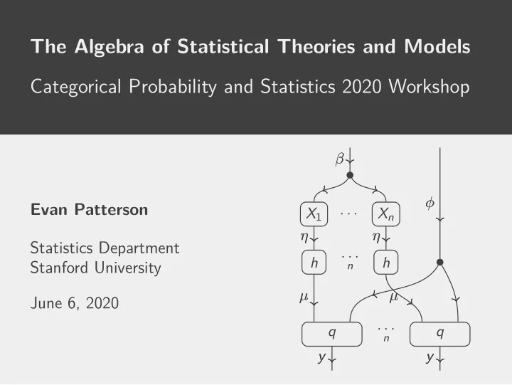
The Algebra of Statistical Theories and Models Categorical Probability and Statistics 2020 Workshop

X1 · · · Xn h · · ·

n

h q · · ·

n

q β φ η η µ µ y y

Evan Patterson Statistics Department Stanford University June 6, 2020

Structuralism about statistical models

Statistical models (1) are not black boxes, but have meaningful internal structure (2) are not uniquely determined, but bear meaningful relationships to alternative, competing models (3) are sometimes purely phenomenological, but are often derived from, or at least motivated by, more general scientific theory This project aims to understand (1) and (2) via categorical logic. In this talk, I assume some knowledge of category theory but as little as I can about statistics.

Statistical models, classically

A statistical model is a parameterized family {Pθ}θ∈Ω of probability distributions on a common space X: Ω is the parameter space X is the sample space Think of a statistical model as a data-generating mechanism P : Ω → X. Statistical inference aims to approximately invert this mechanism: find an estimator d : X → Ω such that, for any θ ∈ Ω, d(X) ≈ θ given data X ∼ Pθ.

Statistical models, classically

This setup goes back to Wald’s statistical decision theory (Wald 1939; Wald 1950). Within it, one can already: define general concepts like sufficiency and ancillarity establish basic results like the Neyman-Fisher factorization and Basu’s theorem Recently, Fritz has shown that much of this may be reproduced in a purely synthetic setting (Fritz 2020) However, the classical definition of statistical model abstracts away a large part of statistics: (1) formalizes models as black boxes (2) does not at all formalize relationships between different models

Logical theories and models

Can logic help formalize the structure of statistical models? Mathematical logic distinguishes between theories and models: Logical theory Model of theory Axiomatic Constructed Synthetic/qualitative Analytic/quantitative Formal language Informal mathematics (usually) Machine representable Not (directly) representable What about statistical theories and statistical models?

Models in logic and in science

Not a new idea to draw a connection between models in logic and in statistics (or in science generally). I claim that the concept of model in the sense of Tarski may be used without distortion and as a funda- mental concept in all of the disci-

• plines. . . In this sense I would assert

that the meaning of the concept of model is the same in mathematics and the empirical sciences. The difference to be found in these disciplines is to be found in their use of the concept. (Suppes 1961) Patrick Suppes (1922–2014)

The semantic view of scientific theories

Suppes initiated the “semantic view” of scientific theories: Many different flavors, from different philosophers (van Fraassen, Sneed, Suppe, Suppes, . . . ) For Suppes, “to axiomatize a theory is to define a set-theoretical predicate” (Suppes 2002) Difficulties for statistical models and beyond: After Suppes, proponents of the semantic view paid little attention to statistics Set theory is impractical to implement, esp. with probability Hard to make sense of relationships between logical theories

The algebraization of logic

Beginning with Lawvere’s thesis (Lawvere 1963), categorical logic has achieved an algebraization of logic: Logical theories are replaced by categorical structures Obliterates the distinction between syntax and semantics Some consequences: Theories are invariant to presentation Functorial semantics, especially outside of Set “Plug-and-play” logical systems, via different categorical gadgets Theories have morphisms, which formalize relationships

Dictionary between category theory, logic, and statistics

Category theory Mathematical logic Statistics Category T Theory Statistical theory* Functor M : T → S Model Statistical model Natural transformation α : M → M′ Model homomorphism Morphism of statistical model

*Statistical theories (T, p) have extra structure, the sampling morphism p : θ → x

Family tree of categorical logics

symmetric monoidal category (symmetric monoidal theory) cartesian category (algebraic theory) regular category (regular logic: ∃, ∧, ⊤) coherent category (coherent logic: ∃, ∧, ∨, ⊤, ⊥) elementary topos (first- and higher-order logic) cartesian closed category (typed λ-calculus with ×, 1) bicartesian closed category (typed λ-calculus with ×, +, 1, 0)

Probability and statistics in the family tree

symmetric monoidal category Markov category cartesian category (algebraic theory) linear algebraic Markov category (statistical theory) linear algebraic cartesian category

Informal example: linear models

A linear model with design matrix X ∈ Rn×p has sampling distribution y ∼ Nn(Xβ, σ2In) w/ parameters β ∈ Rp, σ2 ∈ R+. A theory of a linear model (LM, p) is generated by objects y, β, µ, σ2 and morphisms X : β → µ and q : µ ⊗ σ2 → y and has sampling morphism p given by X q β σ2 σ2 µ y Then a linear model is a functor M : LM → Stat.

Markov kernels

Statistical theories will have functorial semantics in a category of Markov kernels. Recall: A Markov kernel X → Y between measurable spaces X, Y is a measurable map X → Prob(Y). Examples: A statistical model (Pθ)θ∈Ω is a kernel P : Ω → X (ˇ Cencov 1965; ˇ Cencov 1982) Parameterized distributions, e.g., the normal family N : R × R+ → R, (µ, σ2) → N(µ, σ2)

• r, more generally, the d-dimensional normal family

Nd : Rd × Sd

+ → Rd,

(µ, Σ) → Nd(µ, Σ).

Synthetic reasoning about Markov kernels

Two fundamental operations on Markov kernels:

• 1. Composition: For kernels M : X → Y and N : Y → Z,

M N X Y Z (M · N)(dz | x) :=

• Y

N(dz | y)M(dy | x)

• 2. Independent product: For kernels M : W → Y and N : X → Z,

M N W X Y Z (M ⊗ N)(w, x) := M(w) ⊗ N(x)

Synthetic reasoning about Markov kernels

Also a supply of commutative comonoids, for duplicating and discarding data. Markov kernels obey all laws of a cartesian category, except one: M X Y

?

= M M X Y Y .

Proposition

Under regularity conditions, a Markov kernel M : X → Y is deterministic if and only if above equation holds.

Markov categories

Markov categories are a minimalistic axiomatization of categories of Markov kernels (Fong 2012; Cho and Jacobs 2019; Fritz 2020). Definition: A Markov category is a symmetric monoidal category with a supply of commutative comonoids x and x , such that every morphism f : x → y preserves deleting: f x y = x .

Constructions in Markov categories

Definition: A morphism f : x → y in a Markov category is deterministic if f x y = f f x y y . Besides (non)determinism, in a Markov category one can express: conditional independence and exchangeability disintegration, e.g., for Bayesian inference (Cho and Jacobs 2019) many notions of statistical decision theory (Fritz 2020)

Linear and other spaces for statistical models

In order to specify most statistical models, more structure is needed. Much statistics happens in Euclidean space or structured subsets thereof: real vector spaces affine spaces convex cones, esp. R+ or PSD cone Sd

+ ⊂ Rd×d

convex sets, esp. [0, 1] or probability simplex ∆d ⊂ Rd+1 Also in discrete spaces: additive monoids, esp. N or Nk unstructured sets, say {1, 2, . . . , k}

Lattice of linear and other spaces

Such spaces belong to a lattice of symmetric monoidal categories: (Cone, ⊕, 0) (CMon, ⊕, 0) (VectR, ⊕, 0) (Set, ×, 1) (AffR, ×, 1) (Conv, ×, 1) Note: Cone is category of conical spaces, abstracting convex cones Conv is category of convex spaces, abstracting convex sets

Supplying a lattice of PROPs

Dually, there is a lattice of theories (PROPs): Th(CBimon) Th(Cone) Th(CComon) Th(VectR) Th(Conv) Th(AffR) Definition: A supply of a meet-semilattice L of PROPs in a symmetric monoidal category (C, ⊗, I) consists of a monoid homomorphism P : (|C| , ⊗, I) → (L, ∧, ⊤), x → Px, and for each object x ∈ C, a strong monoidal functor sx : Px → C with sx(m) = x⊗m, subject to coherence conditions (mildly generalizing Fong and Spivak 2019).

Linear algebraic Markov categories

Definition: A linear algebraic Markov category is a symmetric monoidal category supplying the above lattice of PROPs, such that it is a Markov category. Linear algebraic Markov categories come in the small, as statistical theories in the large, as the semantics of statistical theories

Category of statistical semantics

The linear algebraic Markov category Stat has as objects, the pairs (V , A), a finite-dimensional real vector space V with a measurable subset A ⊂ V as morphisms (V , A) → (W , B), the Markov kernels A → B a symmetric monoidal structure, given by (V , A) ⊗ (V , B) := (V ⊕ W , A × B), I := (0, {0}) and by the independent product of Markov kernels a supply according to whether the subset A is closed under linear/affine/conical/convex combinations, addition, or nothing.

Additivity of normal family

Normal family is additive: if Xi

ind

∼ N(µi, σ2

i ), then

X1 + X2 ∼ N(µ1 + µ2, σ2

1 + σ2 2)

In Stat, additivity is the equation: N R R+ R+ R = N N R R+ R+ R R+ R+ R

Homogeneity of normal family

Normal family is homogeneous: if X ∼ N(µ, σ2), then cX ∼ N(cµ, c2σ2), ∀c ∈ R. In Stat, homogeneity is the equation: c c2 N R R+ R+ R R+ R+ R = N c R R+ R+ R R ∀c ∈ R. Call both properties together “linear-quadratic”.

Presenting the normal family

Isotropic normal family can be presented by generators and relations.

Theorem

For any d ≥ 1, a linear algebraic Markov category C, containing a morphism f : y⊗d ⊗ s → y⊗d, can presented such that for any supply preserving functor M : C → Stat with M(y) = R and M(s) = R+, the Markov kernel M(f ) : Rd × R+ → Rd is the isotropic normal family, up to an absolute scale. That is, there exists σ2

0 ∈ R+ such that

M(f )(µ, φ) = Nd(µ, φσ2

0Id),

∀µ ∈ Rd, φ ∈ R+.

Characterizations of normal distribution

Main ingredient is the symmetry of the normal distribution.

Theorem (Maxwell)

For any d ≥ 2, a random vector Y ∈ Rd has i.i.d. centered normal distribution if and only if Y is spherically symmetric and has independent components. Or, simpler:

Theorem (P´

• lya 1923)

If X and Y are i.i.d. random variables such that X d = 1 √ 2(X + Y ), then X is centered normal.

Sketch of presentation

• 1. Reduce to centered case via generator g : s → y⊗d:

f y⊗d y⊗d s y⊗d y⊗d

=

g s y⊗d y⊗d

• 2. Assert that g is homogeneous, in above sense
• 3. Assert that g has independent (or i.i.d.) components
• 4. Axiomatize Maxwell’s or P´
• lya’s theorem, e.g., when d = 2,

g s y y

=

g

1 √ 2

s y y

Statistical theories and models

A statistical theory (T, p) consists of a small linear algebraic Markov category T a morphism p : θ → x in T, the sampling morphism A model of a statistical theory (T, p) is a supply preserving functor M : T → Stat. Ω := M(θ) is the parameter space X := M(x) is the sample space P := M(p) : Ω → X is the sampling distribution Note: Statistical theories generally have many different models.

A few simple statistical theories

Example: The initial statistical theory (T, p) is freely generated by

• ne morphism p : θ → x on discrete objects θ and x.

Observation

Every statistical model P : Ω → X is a model of the initial theory. Example: The theory of n i.i.d. samples (T, p) is freely generated by

• ne morphism p0 : θ → x on discrete objects θ and x, with

p θ x⊗n x⊗n := p0 · · ·

n

p0 θ x x .

Theory of a linear model

The theory of a linear model (LM, p) is generated by vector space objects β, µ, and y conical space object σ2 linear map X : β → µ, i.e., morphism X : β → µ subject to equations of linearity and determinism linear-quadratic morphism q : µ ⊗ σ2 → y with sampling morphism p : β ⊗ σ2 → y given by X q β σ2 σ2 µ y

Linear models, as models of a theory

The standard models M : LM → Stat are linear models: M(y) = M(µ) = Rn for some dimension n M(β) = Rp for some dimension p M(σ2) = R+ M(q) : Rn × R+ → Rn is isotropic normal family XM := M(X) : Rp → Rn is arbitrary linear map The sampling distribution is then M(p) : Rp × R+ → Rn (β, σ2) → Nn(XMβ, σ2In) Another model is a weighted linear model where, for fixed VM ∈ Sp

+,

M(p) : (β, σ2) → Nn(XMβ, σ2VM).

Bayesian statistical theories and models

A Bayesian statistical theory (T, p, π) consists of a statistical theory (T, θ

p

− → x) a morphism I

π

− → θ, the prior morphism A model of a Bayesian theory (T, p, π) is a model M : T → Stat of the underlying statistical theory. M(p) is the sampling distribution M(π) is the prior M(π · p) is the marginal or prior predictive distribution

Morphisms of statistical models

A model homomorphism between models M and M′ of a statistical theory (T, p) is a monoidal natural transformation T Stat

M M′ α

Proposition

The components αx : M(x) → M′(x) of model homomorphism are supply homomorphisms. In particular, they are deterministic.

Morphisms of linear models

Let M, M′ be linear models, as models of (LM, p), with designs XM := M(X) ∈ Rn×p, XM′ := M′(X) ∈ Rn′×p′.

Proposition

A model homomorphism α : M → M′ is uniquely determined by linear maps A := αy ∈ Rn′×n and B := αβ ∈ Rp′×p such that AA⊤ ∝ In′ and AXM = XM′B.

Symmetries of statistical models

Corollary

An isomorphism of linear models α : M ∼ = M′, with n = n′ and p = p′, is uniquely determined by linear maps A := αy ∈ CO(n) and B := αβ ∈ GL(p, R) such that XM′ = AXMB−1. Symmetry and invariance is a classical topic in statistics. Advantages

• f our account:

it does not assume identifiability of model (or loss function) it is not restricted to automorphisms or even isomorphisms it ensures that transformations preserve all structure specified by the theory, not just parameter and sample spaces it makes symmetry a property of the theory and model, not an extra structure added arbitrarily

Equivariance of linear regression

Ordinary-least squares (OLS) linear regression is equivariant under model isomorphism (a classical result) “laxly” equivariant under model homomorphism

Theorem

Let α : M → M′ be a homomorphism of linear models. For any y ∈ Rn and β ∈ Rp, if y′ := αy(y) and β′ := αβ(β), then XM′β′ − y′ ≤ aXMβ − y, where a := √ασ2 ∈ R+. In particular, if α is an isomorphism, then ˆ β ∈ argmin

β∈Rp XMβ − y

implies ˆ β′ ∈ argmin

β′∈Rp′ XM′β′ − y′.

Another theory of a linear model

The theory of a linear model on n samples (LMn, pn) is generated by vector spaces β, µ, and y and a conical space σ2 linear maps X1, . . . , Xn : β → µ, a linear-quadratic morphism q : µ ⊗ σ2 → y with sampling morphism pn : β ⊗ σ2 → y⊗n given by X1 q · · ·

n

Xn q β σ2 σ2 µ y µ y

Linear models on n samples

A linear model M : LMn → Stat now assigns M(y) = M(µ) = R M(q) = N : R × R+ → R, the univariate normal family Let M, M′ be linear models on n samples, as models of (LMn, pn), with designs (XM,i)n

i=1 ∈ Rn×p and (XM′,i)n i=1 ∈ Rn×p′.

Proposition

A model homomorphism α : M → M′ is uniquely determined by a scalar a := αy ∈ R and a matrix B := αβ ∈ Rp′×p such that aXM,i = XM′,iB, ∀i = 1, . . . , n.

More theories of a linear model

Theories of a linear model include (LM, p), of a general linear model (LMn, pn), of a LM on n observations (LMp, qp), of a LM on p predictors (LMn,p, qn,p), of a LM on n observations and p predictors Which theory is the right one? Wrong question. Different theories allow different models and model homomorphisms Yet they are related by morphisms of theories

Morphisms of statistical theories

Definition: A (strict) morphism of statistical theories F : (T, p) → (T′, p′) is a supply preserving functor F : T → T′ such that F(p) = p′. The theory morphism induces a model migration functor F ∗ : Mod(T′) → Mod(T) (cf. Spivak 2012) by pre-composition: T′ Stat

M F ∗

→ T T′ Stat

F F ∗(M) M

Morphisms between theories of linear model

Different theories of linear models are related by theory morphisms: (LM, p)

general LM

(LMn, pn)

LM with n observations

(LMp, qp)

LM with p predictors

(LMn,p, qn,p)

LM with n observations and p predictors Fn Gp Fn,p Gn,p

Morphism between two theories of linear model

A theory morphism Fn : (LM, p) → (LMn, pn) sends µ to µ⊗n and y to y⊗n splits the design matrix by rows: Fn :

X β µ

→

X1 · · · Xn β µ µ

splits the morphism q accordingly: Fn :

q µ σ2 σ2 y

→

· · ·

n

q · · ·

n

q σ2 σ2 µ µ y y

preserves the other generators

Theory of a generalized linear model

A theory of a GLM on n samples (GLMn, pn) is generated by vector spaces β and η, a convex space µ, and a conical space φ a discrete object y maps g : µ → η (link function) and h : η → µ (mean function), which are mutually inverse: g h µ η µ = µ and h g η µ η = η . linear maps X1, . . . , Xn : β → η a morphism q : µ ⊗ φ → y

Theory of a generalized linear model

The sampling morphism pn : β ⊗ φ → y⊗n is X1 · · · Xn h · · ·

n

h q · · ·

n

q β φ η η µ µ y y

Morphism between theories of GLM and LM

Fact: “A linear model is a special case of a generalized linear model.” Formally, a theory morphism Gn : (GLMn, pn) → (LMn, pn) sends both µ and η to µ, sends both g and h to the identity 1µ: Gn : g µ η , h η µ → µ sends φ to σ2 preserves the other generators Induces a model migration functor G∗

n : Mod(LMn) → Mod(GLMn).

Lax morphisms of statistical theories

A weaker notion of theory morphism allows for expansion of parameter and sample spaces (cf. McCullagh 2002). A lax* morphism of statistical theories (T, θ

p

− → x) and (T′, θ′ p′ − → x′) consists of a functor F : T → T′ a morphism f0 : θ′ → F(θ) in T′ a morphism f1 : x′ → F(x) in T′ such that the diagram commutes: θ′ x′ Fθ Fx

p′ f0 f1 Fp

*Called “colax”, not “lax,” in (Patterson 2020)

Samples of different sizes as lax theory morphisms

Recall the theory of n i.i.d. samples (T, pn). For any numbers m ≤ n, projection gives a lax theory morphism (1T, 1θ, πm,n−m) : (T, pm) → (T, pn), where laxness condition is p0 · · ·

m

p0 θ x x = p0 · · ·

m

p0 p0 · · ·

n−m

p0 θ x x x x .

Conclusion

Summary:

• 1. introduced statistical theories in style of categorical logic
• 2. recovered statistical models as models of statistical theories
• 3. obtained notion of statistical model homomorphism
• 4. formalized relationships using morphisms of statistical theories
• 5. accompanied by model migration functors

Future work: lots! mathematical investigation of linear algebraic Markov categories compositionality of statistical theories and models software and integration with probabilistic programming

Outlook

How can statistics support scientific theories and models broadly? Traditionally, statistics has emphasized the formal testing of null hypotheses, as if they exist in isolation Rather, science involves an intricate web of interconnected theories, models, experiments, and data Again, a long precedent in philosophy of science: [E]xact analysis of the re- lation between empirical theories and relevant data calls for a hierarchy of models of different logical

• type. (Suppes 1966)

Suppes’ hierarchy of models:

• 1. theoretical model
• 2. model of the experiment
• 3. data model [roughly, a

statistical model] How to make mathematics and statistics out of such ideas?

Thanks!

Main reference is my PhD thesis (Patterson 2020) Available at https://www.epatters.org/papers/ Many more examples of statistical theories and models:

◮ contingency tables ◮ simple Bayesian and hierarchical models ◮ linear mixed models ◮ generalized linear (mixed) models ◮ ...

References I

ˇ Cencov, N. N. (1965). “The categories of mathematical statistics”. Dokl. Akad. Nauk SSSR 164.3. In Russian, pp. 511–514. – (1982). Statistical decision rules and optimal inference. Translations of Mathematical Monographs 53. American Mathematical Society. Cho, Kenta and Bart Jacobs (2019). “Disintegration and Bayesian inversion via string diagrams”. Mathematical Structures in Computer Science 29.7,

• pp. 938–971. doi: 10.1017/S0960129518000488.

Fong, Brendan (2012). “Causal theories: A categorical perspective on Bayesian networks”. MSc thesis. University of Oxford. arXiv: 1301.6201. Fong, Brendan and David I. Spivak (2019). “Supplying bells and whistles in symmetric monoidal categories”. arXiv: 1908.02633. Fritz, Tobias (2020). “A synthetic approach to Markov kernels, conditional independence and theorems on sufficient statistics”. Advances in Mathematics 370.107239. doi: 10.1016/j.aim.2020.107239. arXiv: 1908.07021.

References II

Lawvere, F. William (1963). “Functorial semantics of algebraic theories”. Republished in Reprints in Theory and Applications of Categories, No. 5 (2004),

• pp. 1–121. PhD thesis. Columbia University.

McCullagh, Peter (2002). “What is a statistical model?” Annals of Statistics 30.5,

• pp. 1225–1267. doi: 10.1214/aos/1035844977.

Patterson, Evan (2020). “The algebra and machine representation of statistical models”. PhD thesis. Stanford University. P´

• lya, Georg (1923). “Herleitung des Gaußschen Fehlergesetzes aus einer

Funktionalgleichung”. Mathematische Zeitschrift 18.1, pp. 96–108. doi: 10.1007/BF01192398. Spivak, David I. (2012). “Functorial data migration”. Information and Computation 217, pp. 31–51. doi: 10.1016/j.ic.2012.05.001. arXiv: 1009.1166.

References III

Suppes, Patrick (1961). “A comparison of the meaning and uses of models in mathematics and the empirical sciences”. The concept and the role of the model in mathematics and natural and social sciences, pp. 163–177. doi: 10.1007/978-94-010-3667-2_16. – (1966). “Models of data”. Studies in logic and the foundations of mathematics,

• pp. 252–261. doi: 10.1016/S0049-237X(09)70592-0.

– (2002). Representation and invariance of scientific structures. Online edition. CSLI Publications. Wald, Abraham (1939). “Contributions to the theory of statistical estimation and testing hypotheses”. The Annals of Mathematical Statistics 10.4, pp. 299–326. doi: 10.1214/aoms/1177732144. – (1950). Statistical decision functions. Wiley.