Telescopes & Mirrors Telescopes & Mirrors Giovanni Pareschi - - PowerPoint PPT Presentation

Telescopes & Mirrors Telescopes & Mirrors

Giovanni Pareschi INAF - Osservatorio Astronomico di Brera Via E. Bianchi 46 23807 Merate - Italy E-mail: giovanni.pareschi@brera.inaf.it

 remarks on grazing – incidence for X-ray astronomy

• why grazing incidence reflection
• optical configurations for grazing-incidence mirrors

 making mirrors

• the replication method

examples of past and future X-ray telescopes  remarks on Gamma ray focusing telescopes and optics

Outline Outline

Advantages of focusing optics versus direct-view Advantages of focusing optics versus direct-view detectors detectors

E A B

T n F

eff

Δ =

int min

2

σ

E T A BA n F

eff d

Δ =

int min σ

Moreover: much better imaging capabilities!

B =background flux, Tint = integration time, ΔE = integration bandwidth

Simulation of two sources in a Simulation of two sources in a “ “Einstein Einstein” ” field as seen by a direct view detector field as seen by a direct view detector

With the direct vie detector the second “weak” sources is lost in the background

X-ray astronomical optics history in pills (I) X-ray astronomical optics history in pills (I)

• 1895: Roentgen discovers “X-rays”
• 1948: First succesfull focalization of an X-ray beam by a total-reflection
• ptics (Baez)
• 1952: H. Wolter proposes the use of two-reflection optics based on conics

for X-ray microscopy

• 1960: R. Giacconi and B. Rossi propose the use of grazing incidence optics

for X-ray telescopes

• 1962: discovery by Giacconi et al. of Sco-X1, the first extra-solar X-ray

source

• 1963: Giacconi and Rossi fly the first (small) Wolter I optics to take images
• f Sun in X-rays
• 1965: second flight of a Wolter I focusing optics (Giacconi + Lindslay)
• 1973: SKYLAB carry onboard two small X-ray optics for the study of the Sun

• 1978: Einstein, the first satellite with optics entirely dedicated to X-rays
• 1983: EXOSAT operated (first European mission with X-ray optics aboard)
• 1990: ROSAT, first All Sky Survey in X-rays by means of a focusing

telescope with high imaging capabilities

• 1993: ASCA, a multimudular focusing telescope with enhanced effective area

for spectroscopic purposes

• 1996: BeppoSAX, a broad-band satellite with Ni electroformed optics
• 1999: launch of Chandra, the X-ray telescope with best angular resolution,

and XMM-Newton, the X-ray telescope with most Effective Area

• 2004: launch of the Swift satellite devoted to the GRBs investigation (with

aboard XRT)

• 2005: launch of Suzaku with high throughput optics for enhanced

spectroscopy studies with bolometers

X-ray astronomical optics history in pills (II) X-ray astronomical optics history in pills (II)

Imaging experiments using Bragg reflection from Imaging experiments using Bragg reflection from “ “replicated replicated” ” mica pseudo-cylindrical optics mica pseudo-cylindrical optics

• E. Fermi – Thesis of Laurea, “Formazione di immagini con

i raggi Roentgen” (“Imaging formation with Roentgen rays”), Univ. of Pisa (1922)

Thanks to Giorgio Palumbo!

X-ray optical constants X-ray optical constants

ñ = n + iβ = 1 - δ + iβ (µ = 4 π β/λ cm -1)

• complex index of refraction to descrive the interaction X-rays /matter:

Linear abs. coeff.

δ changes of phase

• at a boundary between two materials of different refraction index n1,

n2 reverse of the momentum P in the z direction:

• the amplitute of reflection is described by the Fresnel’s equations:

1 1

2 k h p

→ →

= π

1 1

2 n k λ π =

→

inc z

n p θ

λ π

sin 2

1 4

∝

momentum transfer

1 2 2 1 1 2 2 1 12

sin sin sin sin θ θ θ θ n n n n r p + − =

2 2 1 1 2 2 1 1 12

sin sin sin sin θ θ θ θ n n n n r s + − =

β absorption

• if vacuum is material #1 (n1 = 1)  the phase velocity in the second medium

increases  beam tends to be deflected in the direction opposite to the normal.

• Snell’s law (n1 cosθ1 =n2 cosθ2) to find a critical angle for total reflection:

π ρ δ

λ θ

A

f N r

Av crit 1 2

2 = ≈

λ = wavelenght ρ = density A = atomico weight f1 = scattering coeff. r0 = classical electron radius

• far from the fluorecence edges f1

≈ Z and for heavy elements Z/A ≈ 0.5:

Total X-ray reflection at grazing incidence Total X-ray reflection at grazing incidence

( )

ρ λ θ ) ( 6 . 5 min A arc

crit

≈

0.8 0.6 0.4 0.2 0.0 Riflettività 14 12 10 8 6 4 2 Energia dei fotoni (keV) Ni Au Angolo di incidenza = 0.5 deg

          − =

      ⋅ ⋅ ⋅ λ θ σ π sin n I I R 4

2 0exp

• reflectivity loss due to scattering:

σ = rms microroughn. level

10

• 5

10

• 4

10

• 3

10

• 2

10

• 1

10 Riflettività 6000 5000 4000 3000 2000 1000 Angolo di incidenza [arcsec] Dati sperimentali Modello z(Nickel)=60 nm

Other examples: C, Ni, Au

x y

y2 = 2 p x

p = 2 * dist. focus-vertex

X-ray mirrors with parabolic profile

• perfect on-axis focusing
• off-axis images strongly affected by coma

The Abbe sine condition to have coma-free focusing mirrors

Typical blurring

• f a focal spot

due to coma

Coma: off-axis abberation caused by a different magnification of reflected rays, depending on the hitting position at the mirror surface

• Coma free mirrors must satisfy the Abbe sine condition:

The surface defined by the intersection of each input ray with its corresponding output ray (principal or Abbe surface) must be a sphere around the image, i.e.:

. sin sin

2 2 1 1

const h h = = θ θ

The parabolic profile approximately obeys to the Abbe rule only near the vertex, i.e. at normal incidence but not for grazing incidence angles  the parabolic geometry is not optimal for X-ray telescopes

Parabolic mirrors & the Abbe sine condition

• H. Wolter, Ann. Der Phys., NY10,94

Wolter’s solution to the X-ray imaging

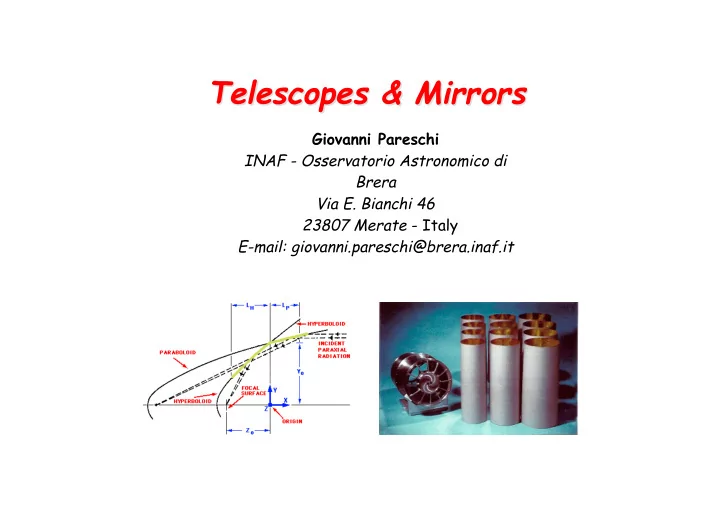
The Wolter I mirror profile for X-ray astronomy applications

• it guarantees the minimum focal length for

a given aperture

• it allows us to nest together many confocal

mirror shells

• Effective Area: 8 π F L θ2 Refl.2

F= focal length = R / tan 4θ

θ= on-axis incidence angle R = aperture radius

The Abbe condition and the Wolter I mirror profile The Abbe condition and the Wolter I mirror profile

θ γ θ γ σ

2 2

tan tan 4 tan tan 2 . +       = F L

rms

σrms = rms blur circle θ = incidence angle γ = off-axis angle L = mirror height F= focal length Spherical aberration term Residual coma term

NOTE: the optimal focal plane is not flat:

r = focal plane radius

θ δ

2 2 2

tan 1 F L r

flat ∝

Alternative profiles derived from Alternative profiles derived from Wolter Wolter I I

• Wolter-Schwarzschild profile: it exactly satisfies the Abbe

sine condition and it has been adopted for the Einstein mirrors; is coma free but it strongly affected by spherical aberration

• double-cone profile: it better approximates the Wolter I at

small reflection angles: It is utilized for practical reasons (- cost + effective area). Intrinsic on-axis focal blurring given by:

F LR HEW

2

∝

• polynomial profile: parameters have been specifically optimized to

maintain the same HEW in a wide field of view

(introducing small aberration on-axis the off-axis imaging behavior is improved  same principle of the Ritchey-Chretienne normal-incidence telescope in the optical band)

• parabolic-profile curved mirrors in just one

direction  to focus a beam in a single point another identical mirror has to be orthogonally placed with respect to the first one;

• it is possible to nest many confocal mirrors to

increase the effective area;

• compared to a Wolter I system with same

focal length and same incidence angle (on-axis), angles are two time larger; NB: by means of a K-B optics was performed the first successful attempt

• f the focalization of an X-ray beam in total-reflection regime (1948)
• imaging capabilities result to be limited by

some inherent aberration;

Kirpatrick Kirpatrick-Baez Telescopes

• Baez Telescopes

• system similar to spherical normal-incidence mirrors

but, in this case, the beam impinges on the convex part

• f the entrance pupil;
• the pupil is formed by a system o channels with

square section uniformly distributed around a spherical surface of radius R. To be focused in a single point a collimated beam has to sustain the reflection by two

• rthogonal walls of a same channel;
• the photons are focused onto points distributed on a

spherical surface of radius R/2;

• a preferential optical axis does not exist  the

system field of view can be in principle as large as 4 p with the same Effective Area for every direction

Lobster-Eye optics

Manufacturing techniques utilized so far

1. Classical precision optical polishing and grinding Projects: Einstein, Rosat, Chandra Advantages: superb angular resolution Drawbacks: high mirror walls   small number of nested

mirror shells, high mass, high cost process

2. Replication Projects: EXOSAT, SAX, JET-X/Swift, XMM, ABRIXAS (

examples follow hereafter)

Advantages: good angular resolution, high mirror “nesting”

the same mandrels for many modules

Drawbacks: relatively high cost process; high mass/geom. area

ratio (if Ni is used).

3. “Thin foil mirrors” Projects: BBXRT, ASCA, SODART, ASTRO-E Advantages: high mirror “nesting” possibility, low mass/geom. area

ratio (the foils are made of Al), cheap process

Drawbacks: until now low imaging resolutions (1-3 arcmin)

Credits: NASA Credits: ESA Credits: ISAS

New Configuration

Present Astronomical optics technologies: Present Astronomical optics technologies: HEW Vs Mass/geometrical area HEW Vs Mass/geometrical area

Chandra

• Focal length = 10 m
• 1 module, 4 shells
• Coating = Iridium
• Angular Resolution = 0.5 arcsec HPD

Rosat: HPD = 3 arcsec Chandra: HPD = 0.5 arcsec

Chandra: a fantastic angular resolution Chandra: a fantastic angular resolution

X-ray optics by Ni electroforming replication X-ray optics by Ni electroforming replication

BeppoSAX Jet-X/Swift XMM-Newton

ESA credits

Cas A

Now the Ni electroforming approach, born and set-up by Citterio et al. For BeppoSAX is a technology almost of-the-shelf for small/medium size

• missions. It will be used for e-Rosita, SVOM and Polar-X

Beppo-SAX soft X-ray (0.1 Beppo-SAX soft X-ray (0.1 – – 10 keV) concentrators 10 keV) concentrators

GRB970228

• Wolter I double-cone approx. – Au coating
• 4 modules – 30 shells/mod.
• F.L. = 180 cm Max diam = 16.1 cm
• Aeff @ 1 keV = 85 cm2 /module
• HEW= 60 arcsec (corresponding to the two-

cones geom. aberration!)

JET-X (optics ready since1996) / SwiftXRT(2004) optics JET-X (optics ready since1996) / SwiftXRT(2004) optics

Source separation: 20”

• Wolter I profile – Au coating (pathfinder
• f XMM)
• 2 mod. (JET-X) / 1 mod (Swift) – 12

shells/mod.

• F.L. = 350 cm - Max diam = 30 cm
• Aeff @ 1 keV= 150 cm2 /module
• HEW= 15 arcsec

XMM-Newton (operational since dec. 1999) XMM-Newton (operational since dec. 1999)

• Wolter I profile – Au coating
• 3 mod. - 58 shells/mod.
• F.L. = 750 cm - Max diam = 70 cm
• Aeff @ 1 keV= 1500 cm2 /module
• HEW= 15 arcsec

Credits: ESA

Replication methods Replication methods

• Ni electroforming replication

(SAX, JET-X/Swift, XMM, ABRIXAS, e-ROSITA, SIMBOL-X, SVOM/XIAO)

• epoxy replication: EXOSAT

(Be), WFXT (Alumina & SiC prototypes), EDGE/XENIA?

WFXT (feasibility study 1997-1998) WFXT (feasibility study 1997-1998) – – Polynomial mirrors Polynomial mirrors

Test @ Panter-MPE

WFXT (epoxy replication su carrier in SiC) – Ø = 60 cm

• F. L. = 300 cm

HEW = 10 arcsec

The focusing problem in the hard X-ray The focusing problem in the hard X-ray region (> 10 keV) region (> 10 keV)

E

crit

ρ ϑ ∝

but

Wolter I geometry

F = focal length R = reflectivity L = mirror height θ = incidence angle

Aeff ≈ F2 x θc2 x R2

At photon energies > 10 keV the cut-off angles for total reflection are very small also for heavy metals   the geometrical areas with usual focal lengths the geometrical areas with usual focal lengths (> 10 m) are in general (> 10 m) are in general negligible negligible

0.6 o

Focal Length Vs. Diameters for SIMBOL- Focal Length Vs. Diameters for SIMBOL- X and other X-ray telescopes X and other X-ray telescopes

Multilayers

Aeff ≈ F2 x θc2 x R2

E

crit

ρ ϑ ∝

The Formation Flight architecture offers the opportunity to The Formation Flight architecture offers the opportunity to implement long FL telescopes! implement long FL telescopes!

θ

Focal length

θ

Focal length

The formation flight contribution The formation flight contribution

θ

Focal length

Wide band multilayers Wide band multilayers

X-ray supermirrors 1 µm

Beetle Aspidomorpha Tecta; b)

Optical supermirrors in a beetle skin

a)

Top-level scientific requirements Top-level scientific requirements

Energy band: ~0.5 – ≥ 80 keV Field of view (at 30 keV): ≥ 12’ (diameter) On-axis effective area: ≥ 100 cm2 at 0.5 keV ≥ 1000 cm2 at 2 keV ≥ 600 cm2 at 8 keV ≥ 300 cm2 at 30 keV ≥ 100 cm2 at 70 keV ≥ 50 cm2 at 80 keV (goal) Detectors background < 2×10-4 cts s-1cm-2keV-1 HED < 3×10-4 cts s-1cm-2keV-1 LED On-axis sensitivity ≤ 10-14c.g.s.(~0.5 µCrab), 10-40 keV band, 3σ, 1Ms, Line sensitivity at 68 keV < 3 ×10-7 ph cm-2 s-1 (3σ, 1Ms) Angular resolution ≤ 20”(HPD), E < 30 keV ≤ 40”(HPD) @ E = 60 keV (goal) Spectral resolution E/ΔE = 40-50 at 6-10 keV E/ΔE = 50 at 68 keV (goal) Absolute timing accuracy 100 µs (50 µs goal) Absolute pointing reconstruction ~ 3″ (radius, 90%) (2” goal) Mission duration 3 years including commissioning and calibrations (2 years of scientific program) + provision for a possible 2 year extension Total number of pointings > 1000 (first 3 years, nominal mission) 500 (during the possible 2 year mission extension)

Min-Max Diameter 250 - 650 mm Focal Length 20000 mm Mirror Height 600 mm Configuration Wolter I Number of Mirror shells 100 Min-Max incidence angles 0.1° - 0.25° Min-Max wall thickness_ 0.25 - 0.55 mm Total Mirror Mass 287 kg

Simbol-X Optical D Simbol-X Optical Design

esign

_ NB: thickness trend 2 times less XMM-

Newton

Min-Max Diameter 250 - 650 mm Focal Length 20000 mm Mirror Height 600 mm Configuration Wolter I Number of Mirror shells 100 Min-Max incidence angles 0.1° - 0.25° Min-Max wall thickness_ 0.25 - 0.55 mm Total Mirror Mass 287 kg

Simbol-X Optical D Simbol-X Optical Design

esign

_ NB: thickness trend 2 times less XMM-

Newton

Angular resolution for past & future Angular resolution for past & future Hard X-ray Experiments Hard X-ray Experiments

Experiment Experiment Year Year “ “Imaging Imaging” ” technique technique Angular Angular resolution resolution

SAX-PDS 1996 Rocking collimator > 3600 arcsec (collimator pitch) INTEGRAL- IBIS 2002 Coded mask 720 arcsec (mask pitch) HEFT (baloon) 2005 Multilayer

• ptics

> 90 arcsec HEW NUSTAR 2011 Multilayer Optics 40-60 arcsec HEW SIMBOL-X SIMBOL-X 2014 2014 Multilayer Multilayer Optics Optics 15-20 arcsec 15-20 arcsec HEW HEW

Expected Flux Sensitivity Expected Flux Sensitivity

Simbol-X Optics Simbol-X Optics

Focal length : 20 m Shell diameters : 30 to 70 cm Shell thickness : 0.2 to 0.6 mm Number of shells : 100

• Heritage from XMM–Newton : nickel shells obtained by

electroforming replication method; low mass obtained via a reduced thickness of shells

• Coating : multi-layer Pt/C needed for requirement on large

FOV and on sensitivity up to > 80 keV N.B. I: The optics module will have both sides covered with thermal blankets N.B. II: a proton diverter will be implemented

Integration of thin mirror shells Integration of thin mirror shells

.

Integration of thin mirror shells Integration of thin mirror shells

.

Pt C

Multilayer deposition concept Multilayer deposition concept

PSPC 2 shells 1.49 keV Tropic camera, 50 kV, shell 291 PN - shell 291, 50 kV

Calibration of the 2 mirror Calibration of the 2 mirror shell prototype at shell prototype at Panter Panter MPE MPE

Calibration of 2 mirror shell Calibration of 2 mirror shell prototype at prototype at Panter Panter MPE MPE

Energy (keV) HEW (arcsec) 291 shell HEW (arcsec) 295 shell 1.5 23 22.5 8 24 27.5 20 27 29 35 31 49 50 33 49

10

• 1

10 10

1

10

2

10

3

10

4

10

5

10

6

Geometric Area (cm

2

) -- HEW (arcsec) 2020 2010 2000 1990 1980 First Activity Year Einstein EXOSAT Rosat ASCA (4 modules) SAX (4 modules) Chandra XMM (3 modules) Constellation-X (4 modules) XEUS Generation-X (6 modules) Effective Area (cm

2

) HEW (arcsec) Geometric Area and Imaging Resolution (HEW) for past and future X-ray telescopes

Where are we going? Where are we going?

XEUS XEUS

– 1 (1.5) m2 @ 0.2 keV – 5 m2 @ 1 keV – 2 m2 @ 7 keV – 1 m2 @ 10 keV – (0.1) m2 @ 30 keV Effective Area Angular Resolution 5 (2) arcsec @ < 10 keV 10 arcsec @ 40 keV Field-of-View 7 (10) arcmin diameter: WFI, HXI 1.7 arcmin diameter: NFI (3 x10-18) @ 0.2–8 keV; 4_ Sensitivity (cgs)

ITEM ITEM

Requirement Requirement Goal Goal

Angular Resolution (HEW) 5 arcsec 2 arcsec Collecting Area @ 1 keV 5 m2 5 m2 Collecting Area @ 7 keV 2 m2 2m2

XEUS X-ray optics requirements XEUS X-ray optics requirements

N.B. data from the proposal document

Optics mass budget Optics mass budget

Mirrors Support ancillary Total 882 kg 176 kg 238 kg 1296 kg

Optics error budget Optics error budget

Specification (arcsec) Inherent Intrinsic Extrinsic Enviro nment Total Goal 1.4 1.2 0.5 0.5 2 Requirement 1.8 3.7 2 2 5

N.B. data from the proposal document N.B. data from the proposal document

Characteristic Value Pore size 0.6 x 1.5 mm2 Aperture radii 0.67–2.1 m Grazing reflection angles 0.27–0.86 degrees Focal length 35 m Plate scale 170_m/arcsec

Optics Characteristics Optics Characteristics

N.B. data from the proposal document

4.5 m 1.3 m 0.7 m XEUS XMM

2.5 x

Total reflecting surface to be produced

Need of a manufacturing process scalable at a high volume production industrial level!

XEUS Effective Area XEUS Effective Area

X-ray Pore Optics System X-ray Pore Optics System

N.B.:concept introduced by D. Willingale et al, Capri 1994

Double-Cone approximation

Pore Optics technology Pore Optics technology

Credits: ESA & Cosine

Cellular solids: light weight structures with a very high stiffness Cellular solids: light weight structures with a very high stiffness

Foamed Regular cellular structures

Preliminary imaging tests onto Preliminary imaging tests onto two-reflection optics (I) two-reflection optics (I)

Credits: ESA, Cosine, MPE

Collon et al, SPIE Proc 67898, in press (2007)

Alternative approach: hot sluping of thin Alternative approach: hot sluping of thin glass segments glass segments

0.4 mm thick segments 1 tandem (without integration) HEW = 13 arcsec

• 3 petal rings, respectively composed by 12 -24 - 36

petals, arranged on the supporting structure;

• Wolter 1 with focal length 35m; Parabola and

hyperbola are 0.6m long (0.3+0.3); 2 mm x 0.15 mm ribs every ~75 mm;

• The total number of mirror shells is 403 made of

slumped glass with constant thickness (0.15 mm);

Petal Ring # Rmin [mm] Rmax [mm] Mirror Shells number 1 610 988 192 2 1130 1508 123 3 1660 2027 88

Wolter I preliminary design for XEUS (I) Wolter I preliminary design for XEUS (I)

Weight including CFRP Structure ~ 2 tons

Wolter I design effective area Wolter I design effective area

Cold slumping glass approach Cold slumping glass approach

62

K-B “tie” type configuration

Geometry related to fairing dimension L=300 mm + 300 mm 8 equal petals 7 sets of equal blocks for each direction (x, y)_ F=35 m: N1=247 N2=243 _=0.0228 rad F=25 m: N1=180 N2=176 _=0.0365 rad F=20 m: N1=146 N2=141 _=0.0455 rad

4520 mm

63

 Possibility to use vacant space  4 equal modules  6 sets of equal blocks for each direction  F=35 m

− N1=260

N2=258

− _=0,023 rad

 F=25 m

− N1=190

N2=185

− _=0,032 rad

 F=20 m

− N1=151

N2=153

− _=0,04 rad

K-B “chocolate” type configuration

3200 mm

4 5 2 5 m

64

D. Fabricant, L.M. Cohen, P. Gorensrein Mechanical cold shaping technology Mirror mudule 20 X 30 cm F = 3,4 m Effective Area at 1,49 keV 82,2 cm^2 Effective Area at 8,01 keV 9,2 cm^2 HEW 30 arcsec at 1,5 keV

LAMAR telescope (1988) LAMAR telescope (1988)_ _

65

Effective area

 Effective area: K-B vs Wolter I for diffent focal lenght  Pt+C coating

Hard X-ray Focusing by mosaic crystals Hard X-ray Focusing by mosaic crystals

• Bragg diffraction from a crystal lattice  reflectivity peaks at:

2 d sin θ = n λ d typical value of a few Angstroms

• mosaic crystals: at microscopic level a structure of microcrystals almost-

parallel to the external crystal surface. The distribution of the crystallites normals is described by a Gaussian law

• each crystallite reflects in an independent way (without any interferometric

coupling with the beams reflected from the other crystallites)  the integrated reflectivity results to be much larger (>100) than for a perfect crystal case

Bragg Laue “

“Bragg Bragg” ” & & “ “Laue Laue” ” Configurations Configurations

FWHM V F f

Gauss eg

×       ∝ µ λ 1 Re

3 2 int

Bragg

e FWHM T V F f

T Gauss eg θ µ

θ λ

sin 3 2 int

sin Re

−

× ×       ∝

Laue

F = Structure Factor V = Volume of the lattice element µ = lin. absorb. coeff

• Focusing optics in the hard X-/soft gamma-ray

band is crucial for a significant leap

• The hard X-ray band (E<80 keV) can be

covered with multilayer mirrors (NuStar, NeXT, Simbol-X) .

• The higher energy band (>80 keV) can be

efficiently covered with Laue lenses.

Why crystal diffraction for high energy telescopes GRI concept

Example of configuration suitable for Example of configuration suitable for GRI low energy lens (200-550 GRI low energy lens (200-550 keV keV) )

3 sigma sensitivity, _T= 106 s

• Crystal material: Cu(111)
• Available mosaic spread: 3-4 arcmin(now also

available with lower spread);

• Crystal tiles supplied by ILL, Grenoble.

Credits;: F. Frontera – University of Ferrara

• Tile size: 15x15x2 mm3
• Mosaic spread: 3-4 arcmin
• Lens support: carbon fiber
• Focal length: 6 m

First lens prototype & light

HEW of 15 arcmin at 200 keV Credits;: F. Frontera – University of Ferrara

• Atmospheric Cherenkov Telescopes permit to perform
• bservations of astronomical objects emitting in gamma-rays with

energies from 50 GeV up to several TeV.

• The showers extend over many kilometers in length and few tens

to hundreds of meters in width and have their maximum located at around 8-12 km altitude. Electrons and positrons in the shower core, moves with ultra-relativistic speed and emits Cherenkov light.

• This radiation is mainly concentrated in the near UV and optical

band and can therefore pass mostly unattenuated to ground and detected by appropriate instruments.

• Light flashes from showers have a very short duration, typically

2-3 ns in case of a g shower.

Chrenkov Atmospheric Telescopes

• Atmospheric Cherenkov Telescopes permit to perform
• bservations of astronomical objects emitting in gamma-rays with

energies from 50 GeV up to several TeV.

• The showers extend over many kilometers in length and few tens

to hundreds of meters in width and have their maximum located at around 8-12 km altitude. Electrons and positrons in the shower core, moves with ultra-relativistic speed and emits Cherenkov light.

• This radiation is mainly concentrated in the near UV and optical

band and can therefore pass mostly unattenuated to ground and detected by appropriate instruments.

• Light flashes from showers have a very short duration, typically

2-3 ns in case of a g shower.

Chrenkov Atmospheric Telescopes

1ES1218 1ES1218 (z=0.18) (z=0.18) New New Source Source

• Davies-Cotton reflector, which is the most commonly used configuration

for TeV telescopes, is used also for Magic

• Originally, the Davies-Cotton telescope was developed as a solar

concentrator and as such, it does not satisfy the rigorous requirements

• f astronomy in the visible wavelength range
• A large reflector composed of many small, identical, spherical facets is

relatively inexpensive to build. The alignment of the optical system is easy.

• A Davies-Cotton telescope consists of a primary mirror with parabolic

approximated configuration, formed by several coronas of spherical mirrors each at different radii; the half of central radius coincides with the Focal Length of the primary

• For Magic the focal length is 34 m and the diameter is 17 m; the

primary is formed by 240 panels of ~ 1 m2 each

The MAGIC Telescope Configuration The MAGIC Telescope Configuration

• Davies-Cotton reflector, which is the most commonly used configuration

for TeV telescopes, is used also for Magic

• Originally, the Davies-Cotton telescope was developed as a solar

concentrator and as such, it does not satisfy the rigorous requirements

• f astronomy in the visible wavelength range
• A large reflector composed of many small, identical, spherical facets is

relatively inexpensive to build. The alignment of the optical system is easy.

• A Davies-Cotton telescope consists of a primary mirror with parabolic

approximated configuration, formed by several coronas of spherical mirrors each at different radii; the half of central radius coincides with the Focal Length of the primary

• For Magic the focal length is 34 m and the diameter is 17 m; the

primary is formed by 240 panels of ~ 1 m2 each

The MAGIC Telescope Configuration The MAGIC Telescope Configuration

• Davies-Cotton reflector, which is the most commonly used configuration

for TeV telescopes, is used also for Magic

• Originally, the Davies-Cotton telescope was developed as a solar

concentrator and as such, it does not satisfy the rigorous requirements

• f astronomy in the visible wavelength range
• A large reflector composed of many small, identical, spherical facets is

relatively inexpensive to build. The alignment of the optical system is easy.

• A Davies-Cotton telescope consists of a primary mirror with parabolic

approximated configuration, formed by several coronas of spherical mirrors each at different radii; the half of central radius coincides with the Focal Length of the primary

• For Magic the focal length is 34 m and the diameter is 17 m; the

primary is formed by 240 panels of ~ 1 m2 each

The MAGIC Telescope Configuration The MAGIC Telescope Configuration

• Geometry:

Parabolic

• Diameter:

17m

• Collecting Area:

240 m2

• F-number (f/D):

1

• FOV:

3.8 deg

• Slew time:

20 s

• Angular resolution:

< 3 arcmin

• Energy Resolution:

30%

• Operating Band:

50 GeV – 50 TeV

• Sensitivity (@1 TeV):

30 mCrab (1 single telescope) 20mCrab (2 telescopes)

• Sensitivity @ 50 GeV:

0.1 Crab (1 single telescope) 0.05 Crab (2 telescopes)

MAGIC Telescope System MAGIC Telescope System

Glass Mirror Manufacturing Glass Mirror Manufacturing

• Derived from a similar technique proposed by for the manufacturing
• f X-Ray optics (XEUS)
• A thin glass sheet (1-2 mm) is elastically deformed so as to retain

the shape imparted by a master with convex profile. If the radius of curvature is large, the sheet can be pressed against the master using vacuum suction

• On the deformed glass sheet (under vacuum force) one glues a

honeycomb structure that provides the needed rigidity

• Then a second glass sheet is glued on the top in order to obtain a

sandwich

• After releasing the vacuum, on the concave side one deposits a

reflecting coating (Aluminum) and a thin protective coating (Quartz)

MASTER HONEYCOMB REFLECTING SHEET BACKING SHEET CURING CHAMBER RELEASE PVD COATING AL + SiO2

Glass Panel Manufacturing flow Glass Panel Manufacturing flow

Master and panel in the making Master and panel in the making

Aluminum master 1040 x 1040 mm

Front and rear of a segment Size = 985 x 985 mm Weight = 9.5 Kg. Nominal curvature radius= 35 m

All 240 panels successfully produced, being installed right now!