Table of contents 1. Introduction: You are already an - - PowerPoint PPT Presentation

Table of contents

74

Conditions Items Ordering items for presentation Judgment Tasks Recruiting participants Pre-processing data (if necessary) Introduction: You are already an experimentalist 1. 2. 3. 4. 5. 6. 7. Plotting 8. Building linear mixed effects models 9. Evaluating linear mixed effects models using Fisher 10. Bayesian statistics and Bayes Factors 12. Validity and replicability of judgments 13. The source of judgment effects 14. Gradience in judgments 15. Section 1: Design Section 2: Analysis Section 3: Application Neyman-Pearson and controlling error rates 11.

Four basic tasks

75

Participants indicate whether a sentence is grammatical/ ungrammatical (possible/impossible, acceptable/ unacceptable). This it technically a two-alternative forced- choice task (2AFC), but I use that label for the next task. Yes-No: Participants judge two (or more) sentences simultaneously, and indicate which is better (or worse). When there are two sentences, it is a two-alternative forced-choice (2AFC). Forced-Choice: Participants judge each sentence individually along a numerical scale. The scale generally has an odd number of points (so there is a middle point), but in theory it could be even. Likert Scale: Participants judge each sentence individually, but judge it relative to a reference sentence. The ratings are numerical. Magnitude Estimation: There are four basic tasks in experimental syntax. I will briefly talk about all of them, but for most experiments, I believe the best choice is Likert Scale.

The Likert Scale Task

76

Participants judge each sentence individually along a numerical scale. The scale generally has an odd number of points (so there is a middle point), but in theory it could be even. Likert Scale: Who thinks that John bought a car? What do you think that John bought? Who wonders whether John bought a car? What do you wonder whether John bought? 1. 2. 3. 4. 1 2 3 4 5 6 7 least acceptable most acceptable For Likert Scale tasks you have to choose the number of scale points. The trick is to choose a number that is high enough for participants to report as many differences as they want, but not so high that they won’t use all of them. I like to use 7. It is also best to use an odd number so there is a middle point. You also need to label the two ends of the scale. I like to use least/most

• acceptable. I also like to make the low numbers the low ratings. The reverse

seems confusing to some participants.

The Likert Scale Task

77

What is the difference between an odd number and an even number of points? I think this question is most salient if you assume (i) a binary grammar (two types of strings: grammatical and ungrammatical), and (ii) a linking hypothesis between acceptability and grammaticality whereby the location on the continuum of acceptability indicates grammaticality (higher is grammatical, lower is ungrammatical). Both of these assumptions are open areas of research — there are plenty of non-binary approaches to grammar; and there are well-known examples of misalignment between acceptability and grammaticality: *The reporter the senator the president insulted contacted filed the story. More people have been to Russian than I have. Unacceptable, but probably grammatical: Initially acceptable, but ungrammatical:

The Likert Scale Task

78

What is the difference between an odd number and an even number of points? An odd number of points gives participants the option of saying that they don’t know whether this should fall on the acceptable or unacceptable side of the spectrum. Who thinks that John bought a car? 1 2 3 4 5 6 7 least acceptable most acceptable Who thinks that John bought a car? 1 2 3 4 5 6 least acceptable most acceptable An even number of points turns this into a type of binary forced-choice: participants have to choose a side of the scale. I like to keep the binary aspect

• ut of the Likert scale because the nature of the relationship between

acceptability and grammaticality is such an open question.

The Likert Scale Task

79

Why 7 points? Why not 5 or 9? Bard et al. 1996 demonstrated that 5 was not enough. Participants can distinguish more than 5 levels of acceptability. To my knowledge, nobody has demonstrated that 7 is not enough, or that some higher number is preferable. This is a gap in our methodological knowledge. But a bit later in this lecture, I will show you that completely unconstrained scales do not increase statistical power over 7 point scales… suggesting that there is a finite number that is ideal. And, I can tell you that I have never had a participant tell me that they felt constrained by a 7 point scale. I only ran in-person studies from 2004 to 2010. Since 2010, nearly all of my experiments have been online, so there is little

• pportunity for them to tell me (unless they email me).

LS Benefit: Effect sizes

80

One of the primary benefits of LS tasks is that they provide a clear mechanism for assessing the sizes of differences between conditions s2 s3 s4 s5 s1 participant 1: 1 2 3 4 5 6 7 There will be some variability in the cases where a sentence falls on the boundary between two ratings (the way that s3 falls on the 4/5 boundary), but in general, the numerical ratings of LS tasks lend themselves to the types of analyses that we want for factorial designs. However, this rests on several assumptions about how participants use the

• scales. Can you think of what those assumptions are? We will go through them

in the “drawbacks” slides for LS!

LS Benefit: Multiple comparisons

81

Even though each sentence is rated in isolation in an LS task, because those ratings are made relative to a scale, it is possible to make comparisons between any and all of the sentences in the experiment. s2 s3 s4 s5 s1 participant 1: 1 2 3 4 5 6 7 This means that you do not need to know which comparisons you are going to make before you run the experiment. Although in practice, there is no point in running an experiment if you don’t know what you are looking for!

LS Benefit: Location on the scale

82

The responses in LS tasks tell you where along the scale a given sentence is. This means that you can interpret the location on the scale if you want to. s2 s3 s4 s5 s1 participant 1: 1 2 3 4 5 6 7 For example, if you assume a binary theory of grammaticality, you could interpret the location of the rating as indicative of the grammaticality of the sentence: grammaticality: Of course, this rests on a number of assumptions about how the participant uses the scale, how grammars work, and how acceptability maps to grammaticality (a linking hypothesis)! So it isn’t an argument, but rather an assumption, or better yet, a research question.

LS Drawback: Scale biases

83

Different participants might choose to use a scale in different ways. s2 s3 s4 s5 s1 participant 1: 1 2 3 4 5 6 7 Scale Bias: participant 2: 3 4 5 participant 3: 1 2 3 participant 4: 5 6 7 We can eliminate basic scale bias with a z-score transformation, which we will talk about a bit later.

LS Drawback: Finite options

84

s2 s1 participant 1: 1 2 3 4 5 6 7 The obvious solution to this is to increase the number of responses in the scale. The LS task gives participants a finite number of response options. This means that there may be certain differences between conditions that they cannot report: The two sentences above would both be rated a 3, even though they do have a small difference between them. But this runs the risk of introducing too many response options. If the scale defines units that are smaller than the units that humans can use, it could introduce noise in the measurements (or stress in the participants).

LS Drawback: Non-linear scales

85

There is no easy solution to this (although one could imagine building a model to try to estimate these non-linearities for each participant). One of the assumptions in the LS task is that each of the response categories is exactly the same size (that they define the same interval). But this need not be the case: s2 s3 s4 s5 s1 participant 1: 1 2 3 4 5 6 7 participant 2: 1 2 3 4 5 6 7 participant 3: 1 2 3 4 5 6 7

The Magnitude Estimation Task

86

Participants judge each sentence individually, but judge it relative to a reference sentence. The ratings are numerical. Magnitude Estimation: Who said my brother was kept tabs on by the FBI? What do you wonder whether John bought? The first step is to define a reference stimulus. Usually this is chosen to be in approximately the middle of the range of acceptability. The reference stimulus is called the standard. It is assigned a number that represents its acceptability rating. This number is called the modulus. Usually the modulus is a nice round number like 100. 100 Participants are then asked to rate each sentence in the experiment relative to the standard and modulus. The idea is that if the sentence is twice as acceptable, they would rate the sentence as twice the modulus (e.g., 200). If it is half as acceptable, they would rate it as half the modulus (e.g., 50): ???

The potential benefits of ME

87

ME was introduced into psychophysics by Stanley Smith Stevens in order to

• vercome two deficiencies in the Likert Scale task. It was introduced to syntax

by Bard et al. (1996) for exactly the same reason. The LS task uses a finite number of responses. In contrast, ME is usually defined over the positive number line, which is countably infinite. ME sidesteps the problem of defining too many responses by tying the response to a multiple of the standard. This could increase precision. 1. There is no guarantee that the intervals in LS tasks are stable (we called these non-linearities earlier). ME eliminates this problem by using the standard as the perceptual unit (a perceptual “inch”). Although this might differ from participant to participant, the responses within participant should be stable. 2. s2 s3 s4 s5 s1 LS: 1 2 3 4 5 6 7 ME: 1x 2x 3x

The cognitive assumptions of ME

88

ME makes two assumptions about the cognitive abilities of participants (see Narens 1996 and Luce 2002): Participants must have the ability to make ratio judgments. 1. The number words (called numerals) that participants use must represent the mathematical numbers (called numbers) that the words denote. 2. Narens (1996) laid out empirical conditions that would test whether these two assumptions hold. He defined them in terms of a magnitude production - a task in which participants must produce a second stimulus that has the right proportion to the first stimulus (e.g., lights). Commutativity: Magnitude assessments are commutative if the order in which successive adjustments (symbolized by ∗ , X is the original stimulus) are made is irrelevant, such that p ∗ (q ∗ X) ≈ q ∗ (p ∗ X). Notice that this makes no reference to numbers (it is about matching the resulting stimuli), so it is only testing the ratio judgment assumption. 1. Multiplicativity: Magnitude assessments are multiplicative if the result of two successive adjustments matches the result of a single adjustment that is the numeric equivalent of the product of the two adjustments, such that p ∗ (q ∗ X) ≈ r ∗ X, when p ⋅ q = r. 2.

Testing commutativity with ME instead of MP

89

Experiment 1 sentence X sentence Y sentence Z 150 200 100 p ∗ (q ∗ X) ≈ q ∗ (p ∗ X) commutativity: (p ∗ X) (q ∗ X) … Experiment 2 sentence Y … … 150 q ∗ (p ∗ X) (p ∗ X) 300 sentence J Experiment 3 sentence Z … … 200 p ∗ (q ∗ X) (q ∗ X) 300 sentence J X If commutativity holds, then both experiment 2 and experiment 3 will yield the same sentence when we look for the p∗q value. The only complicated thing here is that we need to run separate experiments for each participant using the results from experiment 1.

Testing commutativity with ME instead of MP

90

Experiment 1 sentence X sentence Y sentence Z 150 200 100 p ∗ (q ∗ X) ≈ q ∗ (p ∗ X) commutativity: (p ∗ X) (q ∗ X) … Experiment 2 sentence Y … … 100 q ∗ (p ∗ X)/p (p ∗ X)/p 200 sentence J Experiment 3 sentence Z … … 100 p ∗ (q ∗ X)/q (q ∗ X)/q 150 sentence J X We can simplify the process by setting all standards to 100. This allows us to run all three experiments without creating dependencies across the experiments.

Testing commutativity with ME instead of MP

91

The logic of this experiment relies on finding an item that has the correct rating in both experiments 2 and 3. To increase the likelihood of finding that (should commutativey exist), Sprouse 2011 used 8 experiments instead of 3: Experiment 1 sentence 1 sentence 2 sentence 3 100 sentence 4 sentence 5 sentence 6 sentence 7 sentence 8 Experiment 2 sentence 2 sentence 1 sentence 3 100 sentence 4 sentence 5 sentence 6 sentence 7 sentence 8 Experiment 8 sentence 8 sentence 1 sentence 2 100 sentence 3 sentence 4 sentence 5 sentence 6 sentence 7

…

Testing commutativity with ME instead of MP

92

Because of the novelty of this design, and the fact that chance plays such a big role, Sprouse 2011 designed a simulation test to see if the number of matches suggesting commutativity was greater than or less than what would be expected by chance in this design. Basically, a randomization test — which we will discuss in more detail when we do stats later in the course.

identity ±9 ±19 match margin 4 8 12 16 20 24 # of participants p < .05 p < .1 identity ±9 ±19 match margin 4 8 12 16 20 24 # of participants p < .05 p < .1

These figures show the number of participants (out of 24) that show evidence (above chance) of commutativity. Sprouse 2011 ran two experiments, so there are two graphs. The dotted line shows the expected number of participants if acceptability judgments had the same level of commutativity as magnitude estimation in psychophysics.

The problem with ME for acceptability

93

Although there are a number of potential benefits to using ME for psychophysics, it is not clear that these benefits extend to using ME for acceptability judgments because ME for acceptability does not respect the cognitive assumptions of ME (namely, commutativity). Commutativity tests the ability of subjects to make ratio judgments. Sprouse 2011’s results suggest that humans cannot make ratio judgments of acceptability. s2 s3 s4 s5 s1 LS: 1 2 3 4 5 6 7 ME: 1x 2x 3x It seems to me that problem is that ratios require a zero point. Without a zero point, it is impossible to state ratios. Therefore ME requires a zero point. However, it is not clear at all that acceptability has a zero point. What would it even mean for a sentence to have zero acceptability? This lack of meaningful zero point likely causes the breakdown of ME for acceptability.

The Yes-No Task

94

Participants indicate whether a sentence is grammatical/ ungrammatical (possible/impossible, acceptable/ unacceptable). This could also be called a two-alternative forced-choice task, but I reserve that label for the next task. Yes-No: What do you wonder whether John bought? I think that Lisa wrote a book. Who did you meet the man that married? Yes No Yes No Yes No Although I like to call this the yes-no task, this isn’t standardized. Part of the problem is that you could use any pair of categorical labels that you prefer. The other problem is that this is technically an instance of a two-alternative forced-choice task (where the choices are categories).

The Yes-No Task

95

Participants indicate whether a sentence is grammatical/ ungrammatical (possible/impossible, acceptable/ unacceptable). This could also be called a two-alternative forced-choice task, but I reserve that label for the next task. Yes-No: Benefit: If you believe the grammar is binary, then you might also believe that acceptability might reflect that. So, asking people which category sentences belong to could be helpful. Drawback: Participants could have different boundary locations. This will create noise in the ratings for some sentences. participant 1: participant 2: Drawback: This task has less sensitivity to detect differences between sentences that are on the same side of the boundary. This can be problematic for larger designs (e.g. 2x2s).

The Forced-Choice Task

96

Participants judge two (or more) sentences simultaneously, and indicate which is better (or worse). When there are two sentences, it is a two-alternative forced-choice (2AFC). Forced-Choice: What do you wonder whether John bought? What do you think that John bought? You could in principle have as many sentences as you like per group (2AFC, 3AFC, 4AFC); however, I find it difficult to think of a scenario where this would be useful in building a syntactic theory. The fact that one sentence is better than the other two in a 3AFC doesn’t tell you anything about the other two sentences relative to each other. So in practice, this will just be a task for situations when you want to see a difference between two conditions.

FC Benefit

97

The primary benefit of the forced-choice task is that it is explicitly designed to reveal differences between two conditions. If that is the goal of your hypothesis, you can’t get a more perfectly designed task: What do you wonder whether John bought? What do you think that John bought? Notice that the two sentences are the same lexicalization. This means that there is no chance that variability in the lexical items is leading to the difference that is reported by participants. This also means that there is less of a chance that differences in meaning are driving the difference (only differences in meaning that are tied to the structure could be causing the difference). Normally, we don’t recommend using the same lexicalization. But in this case, the paired presentation means that the difference in structure is going to stand

• ut, so we don’t worry about them not noticing it.

FC Drawback: Pre-plan your comparisons

98

One obvious drawback to the forced-choice task is that you can only compare two conditions if they are presented as a pair in the experiment. What do you wonder whether John bought? What do you think that John bought? Who thinks that John bought a car? Who wonders whether John bought a car? 1. 2. 3. 4. If you wanted to compare 1 and 2 or 3 and 4, you’d have to add another pair containing those sentences to your experiment. In practice this means that in order to use a forced-choice experiment, you have to know ahead of time exactly which comparisons you want to make so that you can build them into the design of the experiment.

FC Drawback: No location information

99

Another drawback of the FC task is that it provides no information about where the sentences are on the scale of relative acceptability. s1 s2 Let’s say that you run an FC experiment, and see that two sentence are

• different. They could still be anywhere on the scale:

s1 s2 s1 s2 Option 1: Option 2: Option 3:

FC Drawback: More complicated assembly

100

Because the FC task is predicated upon pairs of sentence, the assembly of the task is a bit more complicated than the other tasks. The first complication is that when you are creating your Latin Squares, you have to keep the pairs of items together. Basically, in an FC task, each “condition” is really a pairing of two sentence types together: list 1 list 2 list 3 list 4 condition 1 1-1 2-2 3-3 4-4 condition 2 2-2 3-3 4-4 1-1 condition 3 3-3 4-4 1-1 2-2 condition 4 4-4 1-1 2-2 3-3

FC Drawback: More complicated assembly

101

The second complication is that you don’t want the two sentence types to appear in the same order each time. Half the time you want the better sentence on top in the pair, and half the time you want the worse sentence on top in the pair. This makes sure that participants can’t take the strategy “always choose top” or “always choose bottom” with any success. So after creating your latin square, you have to go through and make sure that half of the pairs are in one order, and the other half are in the other order: list 1 list 2 list 3 list 4 C1 1-1 2-2 3-3 4-4 C2 2-2 3-3 4-4 1-1 C3 3-3 4-4 1-1 2-2 C4 4-4 1-1 2-2 3-3 Notice that each list/column has two red items first, and two green items first. Notice that each row/condition-pair has two red items first, and two green items first. This is not easy, and I know of no software to automate this.

Comparing Tasks: Qualitative evaluation

102

YN is terrific if you want participants to divide sentences into two groups. But it is not well suited for other types of

• experiments. The boundary increases noise, and makes the

task blind to differences that fall on one side of the boundary. Yes-No: FC is terrific you want to detect a difference between two

• sentences. But it is not well suited for other types of
• experiments. It provides no location information, and can
• nly be analyzed in direct (pre-planned) pairs.

Forced-Choice: LS has the best combination of properties for most

• experiments. It gives effect size information and location

information, and allows for flexible analyses. Its drawbacks are either correctable or mostly theoretical. Likert Scale: Participants can’t do ME of acceptability, so it turns into something like an LS task. I would not use it. Magnitude Estimation:

Comparing Tasks: Statistical Power

103

Statistical power: The probability that a statistical test will favor the alternative hypothesis when the alternative hypothesis is in fact true. This definition will make much more sense later in the course when we discuss

• stats. For now, we can think of it this way: statistical power is the probability
• f detecting a difference between conditions when there really is a difference

between the conditions. It can also be thought of as a measure of sensitivity. As a probability, statistical power ranges from 0 to 1, where 0 means something will never happen, and 1 means it is certain to happen. Probabilities can also be converted to percentages if you like that better: 0% to 100%. Since power is the probability of detecting an effect when one really exists, we want it to be as high as possible… 1 or 100% would be ideal, though in practice this is difficult to achieve (for reasons that we will discuss when we get to stats). In psychology, a good rule of thumb is that .8 or 80% power is a good level of power for a given test.

Comparing Tasks: Statistical Power

104

Statistical power is dependent on a number of factors: The size of the difference to be detected. Larger differences are easier to detect, thus increasing power. So, if you want to compare the statistical power of different tasks, you have to either hold some of these factors constant, or vary some of them to see the impact of different values. Sprouse et al. 2017 did just that for the four tasks that we’ve been discussing. 1. The size of the sample of participants. Larger samples provide better estimates (with less noise), thus increasing power.. 2. The inherent noise in the task. Less-noisy tasks lead to higher power. 3. The rate of false positives that you are willing to tolerate. It is easy to have perfect (1 or 100%) power: just call everything significant! 4.

The phenomena

105

Sprouse et al. 2013 tested 150 phenomena that were randomly sampled from Linguistic Inquiry between 2001 and 2010. Each phenomenon had two conditions: a target condition that was marked unacceptable in the journal article, and a control condition that was marked acceptable. Sprouse et al. 2017 chose 47 of those phenomena to use as critical test cases for comparing power. We chose the 47 to span the lower half of the range of effect sizes. We chose the lower range because that is where the action will be!

• ●
• ●
• small

small small small small small small small small small small small small small small small small small small small small small small small small small small small small small small small small small small small small small small small small small small small small small small small small small small small small small small small small small small small small small small small small small small small small small small small small small small small small small small small small small small small small small small small small small small small small small small small small small small small small small small small small small small small small small small small small small small small small small small small small small small small small small small small small small small small small small small small small medium medium medium medium medium medium medium medium medium medium medium medium medium medium medium medium medium medium medium medium medium medium medium medium medium medium medium medium medium medium medium medium medium medium medium medium medium medium medium medium medium medium medium medium medium medium medium medium medium medium medium medium medium medium medium medium medium medium medium medium medium medium medium medium medium medium medium medium medium medium medium medium medium medium medium medium medium medium medium medium medium medium medium medium medium medium medium medium medium medium medium medium medium medium medium medium medium medium medium medium medium medium medium medium medium medium medium medium medium medium medium medium medium medium medium medium medium medium medium medium medium medium medium medium medium medium medium medium medium medium medium medium medium medium medium medium medium large large large large large large large large large large large large large large large large large large large large large large large large large large large large large large large large large large large large large large large large large large large large large large large large large large large large large large large large large large large large large large large large large large large large large large large large large large large large large large large large large large large large large large large large large large large large large large large large large large large large large large large large large large large large large large large large large large large large large large large large large large large large large large large large large large large large large large large large large

• ●
• ●
• small

small small small small small small small small small small small small small small small small small small small small small small small small small small small small small small small small small small small small small small small small small small small small small small medium medium medium medium medium medium medium medium medium medium medium medium medium medium medium medium medium medium medium medium medium medium medium medium medium medium medium medium medium medium medium medium medium medium medium medium medium medium medium medium medium medium medium medium medium medium medium large large large large large large large large large large large large large large large large large large large large large large large large large large large large large large large large large large large large large large large large large large large large large large large

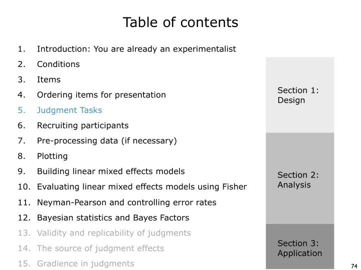
5 10 15 20 5 10 15 20 LI sample from Sprouse et al. 2013 current sample 0.2 0.5 0.8 1 1.5 2 2.5 3 3.5 4 4.5

standardized effect sizes (Cohen's d) count of phenomena

These are standardized effect sizes called Cohen’s d. By standardizing the effect sizes, you can compare across fields!

The experiments and simulations

106

Sprouse et al. 2017 collected 144 participants x 4 tasks (=576) for each of the 47 phenomena. This allowed us to create re-sampling simulations to estimate the statistical power of each task for each phenomenon for sample sizes ranging from 5 to 100. x 1000 choose 5 randomly run a statistical test x 1000 choose 6 randomly run a statistical test x 1000 choose 7 randomly run a statistical test . . . x 1000 choose 100 randomly run a statistical test

Comparing Tasks: Statistical Power

107

These graphs show an estimate of statistical power at each sample size from 5 to 100 (x-axis) for each task (columns) for two types of statistical tests (blue is null hypothesis testing; red is bayes factors). The vertical lines indicate 80%.

Forced−Choice Likert Scale Magnitude Estimation Yes−No

• 30

54

• 16

20

• 11

11

• 8

8

• 37

58

• 17

23

• 11

14

• 34

53

• 18

24

• 11

15

• 53

50

• 25

20

• 16

12

20 40 60 80 100 20 40 60 80 100 20 40 60 80 100 20 40 60 80 100 small medium large extra large 25 50 75 100 25 50 75 100 25 50 75 100 25 50 75 100

sample size mean power (%)

• null

bayes

Comparing Tasks: Statistical Power

108

These graphs show an estimate of statistical power at each sample size from 5 to 100 (x-axis) for each group of phenomena (columns) for two types of statistical tests (rows) for each task (colored lines)

small medium large extra large 20 40 60 80 100 20 40 60 80 100 null bayes 25 50 75 100 25 50 75 100 25 50 75 100 25 50 75 100

sample size mean power (%)

Forced−Choice Likert Scale Magnitude Estimation Yes−No

What we see is the FC has the most power, which is unsurprising given that it is designed to detect differences between conditions. LS and ME are roughly the same, with some minor advantages for LS (matching the findings of Weskott and Fanselow 2011 for some German phenomena). YN has the lowest power (most of the time), which is unsurprising given that it is not designed to detect differences between conditions, but rather categorize sentence types.

Comparing LS and ME: ratings and effect sizes

109

As a quick aside, to substantiate my belief that participants turn ME tasks into LS tasks, we can compare the ratings of the same set of 300 conditions from Sprouse et al. 2013 using each task:

• ●
• ●
• ●
• ●
• ●
• ●
• ●
• r = 0.99

−1 1 −1.0 −0.5 0.0 0.5 1.0

LS ratings (z−transformed) ME ratings (z−transformed)

• ●
• ●
• ●
• ●
• ●
• r = 1

−1 1 2 −1 1 2

LS effect sizes (difference in means) ME effect sizes (difference in means)

The correlations are ridiculous. Pearson’s r ranges from -1 (perfectly negatively correlated) to 1 (perfectly positively correlated). The r’s here are .99 for ratings, and 1 for effect sizes. The ratings slope is .95 and the effect sizes slope is 1, again suggesting a really high degree of equivalence between the two tasks. This suggests the power loss in the previous slides is likely due to the higher variability in ME ratings (because of more response options), as noted by Weskott and Fanselow

• 2011. This is evidence that unlimited response scales are not necessarily ideal.

Instructions

110

It is fairly common for non-linguists to wonder about the instructions that we give participants. I get the sense that in other fields, the instructions can really impact the results. The only systematic study of this that I know is reported in Cowart’s 1997 textbook. He reports that his manipulations of the instructions led to no differences in the pattern of results that he obtained. All he could do was move judgments (of all sentences) up or down on the scale. I’ve never studied this myself, though I’ve also never noticed any artifacts in my results that might suggest a problem with the instructions. I have provided HTML templates for each of these tasks that can be used on Amazon Mechanical Turk (we’ll look at them soon). The instructions that I use are contained in these templates, so you can take a look at them if you’d like some inspiration for instructions for your tasks.