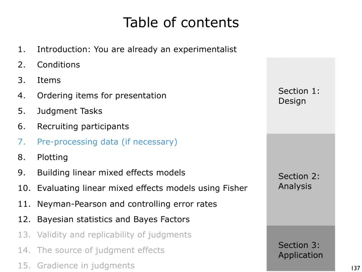
Table of contents 1. Introduction: You are already an - PowerPoint PPT Presentation

Table of contents 1. Introduction: You are already an experimentalist 2. Conditions 3. Items Section 1: 4. Ordering items for presentation Design 5. Judgment Tasks 6. Recruiting participants 7. Pre-processing data (if necessary) 8. Plotting 9. Building linear mixed effects models Section 2: Analysis 10. Evaluating linear mixed effects models using Fisher 11. Neyman-Pearson and controlling error rates 12. Bayesian statistics and Bayes Factors 13. Validity and replicability of judgments Section 3: 14. The source of judgment effects Application 15. Gradience in judgments 137

What is pre-processing Pre-processing is any manipulation you do to your data before the actual statistical analysis. For organizational purposes, I am going to lump two types of pre-processing together in this section, though they are distinct in principle. One type of pre-processing that you will always have to do is data formatting. You need to arrange your data in such a way that you can easily do the analysis (modeling, plotting, etc) that you need to do. Data formatting doesn’t change your data, so you should feel free to do whatever you need to do to make things work. Another type of pre-processing that you may have to do is data transformation. This is where you take your raw data and perform some number of calculations to derive new data (e.g., averaging, z-score transformations, log transformations, or in EEG, filtering). Data transformations should always be theoretically justified, and if possible, kept to a minimum. They change your data! I am going to cover both in this section because (i) they both use R, and (ii) the result is a data file that you can use for statistical analysis and plotting. 138

Formatting your data 139

Two formats: wide and long When humans enter experimental data into a table, they tend to do it in wide format . It is a very intuitive format for data. In wide format , each row represents a participant . Each column represents something about the participant, such as a property or an experimental trial . And each cell contains the value for that property. age trial 1 trial 2 trial 3 trial 4 participant 1 18 2 7 6 1 participant 2 22 2 6 5 1 participant 3 23 3 7 4 2 Wide format has some uses in computer-aided analysis, typically as part of a calculation of a new value; but it is not the dominant format. I would say that I use wide format less than 5% of the time. 95% of the time, the analyses that you will perform will call for long format. 140

Two formats: wide and long When humans enter experimental data into a table, they tend to do it in wide format . It is a very intuitive format for data. In wide format , each row represents a participant . Each column represents something about the participant, such as a property or an experimental trial . And each cell contains the value for that property. Wide format grows longer by one row age trial 1 trial 2 trial 3 trial 4 every time you add a participant, and by one column every time you add a participant 1 18 2 7 6 1 trial/response/measurement/property. Because many experiments will have more trials/responses/properties than participant 2 22 2 6 5 1 participants, the table will often look like a rectangle whose width is participant 3 23 3 7 4 2 greater than its height. Wide format has some uses in computer-aided analysis, typically as part of a calculation of a new value; but it is not the dominant format. I would say that I use wide format less than 5% of the time. 95% of the time, the analyses that you will perform will call for long format. 141

Two formats: wide and long The primary format for computer-aided statistical analysis is long format . At first, long format is less intuitive than wide format, but you will very quickly learn to appreciate its logic. In long format , each row represents a trial . Each column represents a property of that trial, such as the ID of the participant in that trial, the condition of that trial, the item used in that trial, and ultimately the rating (or response) that came from that trial. participant age condition item rating trial 1 1 21 long.island 1 1 trial 2 1 21 short.non 4 7 trial 3 1 21 long.non 2 5 trial 4 1 21 short.island 3 5 142

Two formats: wide and long The primary format for computer-aided statistical analysis is long format . At first, long format is less intuitive than wide format, but you will very quickly learn to appreciate its logic. In long format , each row represents a trial . Each column represents a property of that trial, such as the ID of the participant in that trial, the condition of that trial, the item used in that trial, and ultimately the rating (or response) that came from that trial. Long format is called “long” because it leads to really long tables. Each subject will have a number of rows participant age condition item rating equal to the number of trials in the the experiment. So 40 participants x trial 1 1 21 long.island 1 1 100 items = 4000 rows. Both formats grow longer with additional trial 2 1 21 short.non 4 7 participants, but long format grows longer much faster. And long format trial 3 1 21 long.non 2 5 grows longer with additional trials (wide format grows wider with additional trials). trial 4 1 21 short.island 3 5 143

AMT gives you results in wide format (IBEX gives results in its own hybrid format) But that is ok, we can use R to convert the results to long format. Exercise 6: convert wide format AMT data to long format In the document exercise.6.pdf, I give you a list of functions that you can (and probably will) use to do this. The trick with this, and any script you write, is to start by writing out the steps that you want to achieve in plain English. Then you can figure out how to make R perform those steps. In this case, you are re-arranging the data. So figure out how you would do that (with cutting and pasting, and filling in labels), and then convert those steps to R. 144

There are two solution scripts on the website I’ve created two scripts that can convert wide AMT data to long format: convert.to.long.format.v1.R and convert.to.long.format.v2.R . Version 1 works very similarly to the way you would convert from wide to long if you were cutting and pasting in excel. It cuts away different pieces of the dataset, stacks the columns that need to be stacked, and pastes them back together. Version 2 uses functions from two packages that were specifically designed to make manipulating data easier (including converting from wide format to long format). These packages are tidyr and dplyr. These two packages are now available in a single package called tidyverse. Tidyverse also includes other packages that are useful for data manipulation and visualization, including ggplot2, which we will use next time to make plots! We will go through these later so that you can see what the code looks like. You can also add them to your growing library of R scripts (and use them in future experiments). NEW: My scripts work on AMT data. Brian created a script to convert IBEX data to long format! 145

Next step: adding item information The csv file called results.long.format.no.items.csv contains the results of converting from wide to long format. Although it is technically possible to upload item keys to AMT, and then have the AMT results contain item keys, I typically don’t do that (and IBEX cannot do that). AMT didn’t have the item or condition labels, so we need to add that ourselves. This means we need to add the item keys to our long format dataset. This is where our keys.csv file comes into play. We are going to use it to add item codes to the dataset. Then, we can use R to convert the item codes into condition codes and factors for each item! I have already written a script to add item keys, derive condition codes, and derive factor/level codes. It is called add.items.conditions.factors.r . 146

Next step: Correcting scale bias (z-scores) Recall that pre-processing is any manipulation you do to your data before the actual statistical analysis. As a general rule, you should keep the pre- processing to a minimum (pre-processing changes your data!). But there is at least one property of judgment data that people agree should be corrected before analysis: scale bias . Scale Bias: Different participants might choose to use a scale in different ways. There are two types of scale bias that are relatively straightforward to correct. Skew: Different participants might use different parts of the scale, such as one using the high end, and another the low end). Compression/ Different participants might use different amounts of the Expansion: scale, such as one using only 3/7 responses, and another using the full 7 responses. The best defense against scale bias is a well-designed PRO TIP: experiment. Try to have the mean rating of your items equal the mid-point of your scale. Make sure all of your responses will be used, will be used an equal number of times! 147