SLIDE 1
Waiting for Unruh
Jorma Louko
School of Mathematical Sciences, University of Nottingham
Quantum Field Theory, University of York, 4–7 April 2017
Christopher J Fewster, Benito A Ju´ arez-Aubry, JL
CQG 33 (2016) 165003 [arXiv:1605.01316]
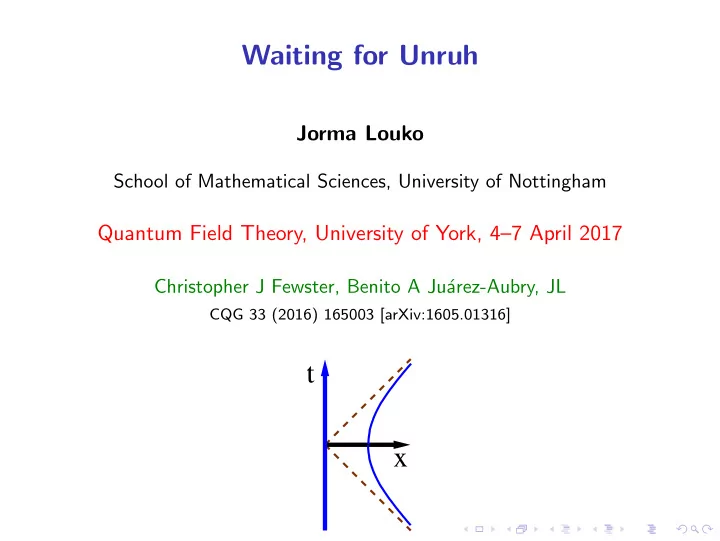
t x
SLIDE 2
Excitation
+ + − −
SLIDE 3
Excitation
+ + − −
SLIDE 4 Plan
◮ Long time limit: adiabatic scaling versus plateau scaling
◮ Unruh-DeWitt
◮ Thermalisation time at large Egap
SLIDE 5
Well established
◮ Uniformly linearly accelerated observer sees Minkowki vacuum
as thermal, T =
a 2π
Unruh 1976
◮ Weak coupling, long time, negligible switching effects ◮ Thermal: Detector records detailed balance:
P↓ P↑ = eEgap/T
SLIDE 6
Well established
◮ Uniformly linearly accelerated observer sees Minkowki vacuum
as thermal, T =
a 2π
Unruh 1976
◮ Weak coupling, long time, negligible switching effects ◮ Thermal: Detector records detailed balance:
P↓ P↑ = eEgap/T
Beyond: non-stationary
◮ Non-uniform acceleration ◮ Curved spacetime: Hawking effect
E.g. detector falling into a black hole
“Time-dependent temperature” ?
SLIDE 7
Our aim
How long does a detector need to operate to record (approximate) detailed balance,
P↓ P↑ = eEgap/T ?
SLIDE 8
Our aim
How long does a detector need to operate to record (approximate) detailed balance,
P↓ P↑ = eEgap/T ?
Novel setting
◮ How long in terms of Egap, at large Egap
− → experiment?
◮ Switching: smooth and compact support ◮ Mathematically precise (nothing hidden in iǫ)
SLIDE 9
Our aim
How long does a detector need to operate to record (approximate) detailed balance,
P↓ P↑ = eEgap/T ?
Novel setting
◮ How long in terms of Egap, at large Egap
− → experiment?
◮ Switching: smooth and compact support ◮ Mathematically precise (nothing hidden in iǫ)
Limitations
◮ Weak coupling −
→ first-order perturbation theory
◮ (3 + 1) Minkowski, massless scalar field (for core results)
SLIDE 10
How long?
Adiabatic switching
τ
λ 1
χ (τ) = χ (τ/λ) λτ
Plateau switching
τ
p
χ (τ)
λ
τs τs λτ Long time: λ → ∞
SLIDE 11
(Unruh-DeWitt)
Quantum field Two-state detector (atom)
(3 + 1) spacetime dimension
φ real scalar field, m = 0 1
|0 Minkowski vacuum x(τ) detector worldline, τ proper time
SLIDE 12
(Unruh-DeWitt)
Quantum field Two-state detector (atom)
(3 + 1) spacetime dimension
φ real scalar field, m = 0 1
|0 Minkowski vacuum x(τ) detector worldline, τ proper time
Interaction
Hint(τ) = cχ(τ)µ(τ)φ
coupling constant χ switching function, C ∞
0 , real-valued
µ detector’s monopole moment operator
SLIDE 13 Probability of transition ⊗ |0 − → 1 ⊗ |anything in first-order perturbation theory: P(E) = c2
- 0µ(0)1
- 2
- detector internals only:
drop!
× F(E)
trajectory and |0: response function
F(E) = ∞
−∞
dτ ′ ∞
−∞
dτ ′′ e−iE(τ ′−τ ′′) χ(τ ′)χ(τ ′′) W (τ ′, τ ′′) W (τ ′, τ ′′) = 0|φ
Wightman function (distribution)
SLIDE 14 Stationary
W (τ ′, τ ′′) = W (τ ′ − τ ′′) F(E) = 1 2π ∞
−∞
dω | χ(ω)|2 W (E + ω)
Unruh
ω 2π
- e2πω/a − 1
- a > 0: proper acceleration
- W (−ω)
- W (ω)
= e2πω/a ⇒ T = a 2π Unruh temperature
SLIDE 15
Theorem 0. With either switching, for any fixed E,
Fλ(E) λ − − − →
λ→∞
(const) × W (E) ⇒ Detailed balance at λ → ∞ (as expected)
SLIDE 16
Theorem 0. With either switching, for any fixed E,
Fλ(E) λ − − − →
λ→∞
(const) × W (E) ⇒ Detailed balance at λ → ∞ (as expected)
Theorem 1. For fixed λ, Fλ(E) is not exponentially suppressed
as E → ∞. ⇒ Detailed balance at λ → ∞ cannot be uniform in E.
SLIDE 17
Theorem 0. With either switching, for any fixed E,
Fλ(E) λ − − − →
λ→∞
(const) × W (E) ⇒ Detailed balance at λ → ∞ (as expected)
Theorem 1. For fixed λ, Fλ(E) is not exponentially suppressed
as E → ∞. ⇒ Detailed balance at λ → ∞ cannot be uniform in E.
Theorem 2. For either switching,
Fλ(−E) Fλ(E) − − − − →
E→∞
e2πE/a with exponentially growing λ(E) ⇒ Detailed balance at large Egap in exponentially long waiting time
SLIDE 18 Theorem 3. For adiabatic switching,
Fλ(−E) Fλ(E) − − − − →
E→∞
e2πE/a (∗) with polynomially growing λ(E), provided
strong falloff
(Cf. Fewster and Ford 2015)
⇒ Detailed balance at large Egap in polynomially long waiting time
SLIDE 19 Theorem 3. For adiabatic switching,
Fλ(−E) Fλ(E) − − − − →
E→∞
e2πE/a (∗) with polynomially growing λ(E), provided
strong falloff
(Cf. Fewster and Ford 2015)
⇒ Detailed balance at large Egap in polynomially long waiting time
Theorem 4. For plateau switching, no polynomially growing
λ(E) gives (∗) ⇒ Detailed balance at large Egap requires longer than polynomial waiting time.
SLIDE 20
Detailed balance in the Unruh effect at Egap → ∞:
◮ (3 + 1) massless scalar ◮ Polynomial waiting time suffices for adiabatically scaled
switching with sufficiently strong Fourier decay
◮ No polynomial waiting time suffices for plateau scaled
switching Upshots:
◮ Large Egap regime has limited relevance for defining a “time
dependent temperature”
◮ Interest for (analogue) experiments?