T Valve TC Plant TS TS - + Feedback Loop TC Steam - - PowerPoint PPT Presentation

Department of Chemical Engineering I.I.T. Bombay, India

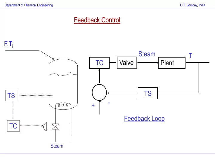
F,Ti TS TC Feedback Control

Steam

Plant T Steam Valve TC TS +

• Feedback Loop

Department of Chemical Engineering I.I.T. Bombay, India

Typical Elements of the Feedback Loop The plant Plant T Steam Valve

Controller Signal (4-20 mA/ 1-5V/ 3-15 psi)

Sensor TS T Tm, mV signal Comparator +

• Setpoint

Error signal, mV Tm

Department of Chemical Engineering I.I.T. Bombay, India

Controller TC Error signal Valve / Actuator TS Controller output % valve opening / steam flowrate Signal to valve Typically valve and sensor dynamics are of simple first order type and are lumped into the plant dynamics. Typical Elements of the Feedback Loop

Department of Chemical Engineering I.I.T. Bombay, India

Controller types for feedback control Proportional Controller c(t) = p(t) -ps = Kc (t) , where c is the controller output, (t) is the error and ps is the output at zero error. In the laplace domain, c(s) = Kc (s) => gc(s) = c(s)/ (s) =Kc Kc is called the proportional gain of the controller and is sometimes represented as proportional band, PB.

variable) measured

• f

range maximum ( K

• utput)

controller

• f

range maximum .( 100

c

PB 

Department of Chemical Engineering I.I.T. Bombay, India

Controller types for feedback control Proportional + Integral Controller where c is the controller output, (t) is the error and ps is the output at zero error.

         



t I c s

dt t t K p t p t c ) ( 1 ) ( ) ( ) (             s K s s c s g

I c c

  1 1 ) ( ) ( ) (

The term I is called the integral time, reset time and the reciprocal is called the reset time.

Department of Chemical Engineering I.I.T. Bombay, India

p

t

Integral action is usually used in conjunction with proportional mode. Interpreted as repetition of the proportional action after every integral time. With valve saturation, reset windup occurs Integral action

Department of Chemical Engineering I.I.T. Bombay, India

Controller types for feedback control Proportional + Integral + Derivative Controller where c is the controller output, (t) is the error and ps is the output at zero error.

          



t D I c s

dt t d dt t t K p t p t c ) ( ) ( 1 ) ( ) ( ) (                s s K s s c s g

D I c c

   1 1 ) ( ) ( ) (

The term D is called the derivative time constant.

Department of Chemical Engineering I.I.T. Bombay, India

Closed Loop Transfer Functions Unlike in the open loop case, the closed loop has two independent inputs, viz. the set point and the disturbance. Assuming that all other elements such as valve and sensors are lumped with the process dynamics, the block diagram can be drawn as,

Plant controller yd +

• y

u disturbance d + +

Department of Chemical Engineering I.I.T. Bombay, India

Closed Loop Transfer Functions From the previous block diagram, the following are true:

) ( ) ( ) ( s s g s u

c

  ) ( ) ( ) ( ) ( ) ( ) ( ) ( ) ( ) ( ) ( s d s g s s g s g s d s g s u s g s y

d c p d p

     ) ( ) ( ) ( s y s y s

d

  

Therefore,

) ( ) ( ) ( 1 ) ( ) ( ) ( ) ( 1 ) ( ) ( ) ( , ) ( ) ( ) ( ) ( ) ( ) ( ) ( ) ( ) ( s d s g s g s g s y s g s g s g s g s y

• r

s d s g s y s g s g s y s g s g s y

c p d d c p c p d d c p c p

      

Servo response Regulatory response

Department of Chemical Engineering I.I.T. Bombay, India

Closed loop response of first order + proportional (P) control

1 1 1 1 1 1 1 1 ) (         s KK KK KK s s KK s KK s y

c c c c c

  

For gp(s)=

1  s K 

and gc(s)=Kc,the response to a unit step at the set point is given by, The system responds like a first order process with a smaller time constant and a gain close to unity. The steady state error between the set point (unit step) and the process output y(t) is called the offset. Most processes under proportional control exhibit offset.

Department of Chemical Engineering I.I.T. Bombay, India

Existence of off-set which decreases with increasing gain. Large gain can also result in instability and amplification

• f noise.

Closed loop response of first order + proportional (P) control

Department of Chemical Engineering I.I.T. Bombay, India

Closed loop response of first order + (PI) control

Ku y dt dy             



t d I d c

dt y y y y K t u ) ( 1 ) ( ) ( 

and

          



t d I d c

dt y y y y KK y dt dy ) ( 1 ) (  

Therefore,

d I c c

y y KK dt dy KK dt y d       ) 1 (

2 2 1

Therefore the closed loop transfer function is second order with lead,

) ( ) 1 ( ) 1 ( ) (

2 1

s y KK s KK s s KK s y

d c c I I I c

        

This could yield oscillatory response with possible overshoot. For a unit step change, it will reach set-point and exhibit zero offset. Integral action therefore increases the effective order of the system but gives zero

• ffset.

Department of Chemical Engineering I.I.T. Bombay, India

Integral action causes off-set to be zero High proportional gain causes oscillatory response High integral action leads to sluggish response

Closed loop response of first order + (PI) control

Department of Chemical Engineering I.I.T. Bombay, India

Closed loop response of first order + (PD) control

Ku y dt dy            dt d K t u

D c

   ) (

and Therefore the closed loop transfer function is first order with lead term,

) ( 1 ) ( ) 1 ( ) ( s y KK s KK s KK s y

d c D c D c

       

The overall order is therefore actually reduced. Transient response will be that of a lead lag system. It will exhibit steady state offset. Likewise for PID control, the closed loop transfer will have 2 poles and 2 zeros and due to integral mode, it will not exhibit offset.

Department of Chemical Engineering I.I.T. Bombay, India

Closed loop response of first order + (PID) control Derivative action leads to stability due the lead term in the transfer function.

Department of Chemical Engineering I.I.T. Bombay, India

Derivative mode illustration : on-off control of a heater.

Department of Chemical Engineering I.I.T. Bombay, India

Period Sign of error Type of current action More or less Corrective action necessary sign of de/dt Effect of derivative action (0,t1) positive heating more decrease heat negative decrease heat (t1,t2) negative cooling less increase cooling negative increase cooling (t2,t3) negative cooling more decrease cooling positive decrease cooling

Anticipatory action of the derivative mode

Department of Chemical Engineering I.I.T. Bombay, India

Integral action and offset removal Consider that at steady state, the steam flow rate is 100 kg/hr and the temperature is 200o C. Suppose that a setpoint change to 205 oC is introduced. Let us now consider how a P and PI controller would behave at steady state in closed loop.

) ( ) ( t K t u

c



The equation is and therefore

dt t d K dt t du

c

) ( ) (  

At steady state, rate of change is zero and therefore

) ( ) (   dt t d dt t du 

This could happen only if  is a zero or a non-zero constant. If  is a zero, the deviation in steam flowrate u will be zero and also error between setpoint and CV is zero. This is not possible physically as you cannot get temperature to rise without supplying additional steam. Therefore,  = 0

Department of Chemical Engineering I.I.T. Bombay, India

Integral action and offset removal

dt t K t K t u

t I c c



  ) ( ) ( ) (   

and therefore

) ( 1 ) ( ) ( t dt t d K dt t du

I c

    

At steady state, rate of change is zero and therefore

) ( ) (   dt t d dt t du 

For PI control, the equation is This means that the error must go to zero at steady state and the extra control effort comes from the integral term. This ensures that a nonzero deviation in the control effort is available through integral action.

Department of Chemical Engineering I.I.T. Bombay, India

Anti-reset wind up schemes

Department of Chemical Engineering I.I.T. Bombay, India

Lectures 14 : Stability with Feedback and Controller Design

Department of Chemical Engineering I.I.T. Bombay, India

Closed Loop Stability

Characteristic Equation ) ( ) ( 1   s g s g

p c

Analysis of the roots of this equation tells us about the stability of the closed loop system. But this is really a function of the controller parameters through the term gc(s) and therefore design methods need to include stability as a first criterion. The stable region is first determined before the controller design task is taken up.

Department of Chemical Engineering I.I.T. Bombay, India

Methods for determining stability

Routh’s Stability Test: tells us how many roots are in the RHP which would thus lead to instability. The test is applicable to polynomials only. Steps 1. Write the characteristic equation in standard form a0sn+ a1sn-1 + a2sn-2 + ….. + an-1s + an = 0 Leading coefficient a0 must be positive. If even one of the coefficient is negative, then at least one root lies in the RHP and the system is unstable. Else,

• 2. Generate the Routh array: This array will have n+1 rows for an nth order
• polynomial. The first two rows can be generated from the characteristic
• equation. The next (n+1-2) rows are generated algebraically.

Department of Chemical Engineering I.I.T. Bombay, India

Routh’s stability test

Routh array Row 1 a0 a2 a4 …

…..

Row 2 a1 a3 a5 …

…..

Row 3 b1 b2 b3 …

…..

Row 4 c1 c2 c3 …

…..

1 5 4 1 2 1 3 2 1 1

and a a a a a b a a a a a b    

1 3 1 5 1 2 1 2 1 3 1 1

and b b a a b c b b a a b c    

Row n+1 z1 The first column must contain all elements that are positive, for stability.

Department of Chemical Engineering I.I.T. Bombay, India

Illustrative examples

Consider the polynomial s4+ 5s3 + 3s2 +1 = 0. What can you say about its stability ? Consider the polynomial 10s3 +17s2 + 8s +1 + Kc =0. What can you say about its stability as a function of Kc? Construct the routh array Row 1 10 8 Row 2 17 1+Kc Row 3 7.41-0.588Kc 0 Row 4 1+Kc System will be stable for –1 < Kc < 12.6

Department of Chemical Engineering I.I.T. Bombay, India

Routh Stability limits

If one of the rows (say n) becomes zero, this means that a pair of purely imaginary roots exist. These can be evaluated from the n-1th row. Limits on the controller gain can therefore be calculated by requiring all the first column elements to be zero. An alternate way of calculating the stability limits is to simply set s=jw and check at what values of K, the roots have positive real parts. For, the polynomial 10s3 +17s2 + 8s +1 + Kc =0, it can be shown that the same limits are obtained.

Department of Chemical Engineering I.I.T. Bombay, India

Effect of model order

) 1 5 )( 1 3 )( 1 ( 15 ) (     s s s s Gplant

1 8 15 ) (

5 . 1

 



s e s G

s ml

Suppose that the following plant is approximated by Apparent mismatch in the dynamics could be more serious than it appears above

Department of Chemical Engineering I.I.T. Bombay, India

Effect of model order

Mismatch is considerable at high frequencies, that is important from control viewpoint.

Department of Chemical Engineering I.I.T. Bombay, India

Stability limits by direct substitution

For, the polynomial 10s3 +17s2 + 8s +1 + Kc =0, set s=jw and solve for the real and imaginary parts. So, -10jw3 +17w2 + 8jw +1 + Kc =0, which yields (1+Kc-17w2) + j(8w-10w3) =0. Setting the real and imaginary components to zero gives 1+Kcm-17w2 =0 and 8w-10w3 = 0 so w2=0.8 or w = ±0.894 and Kc = 12.6 Thus a sustained oscillation of frequency w=0.894 rad/min occurs for Kc=12.6.

Department of Chemical Engineering I.I.T. Bombay, India

Stability Limits by Root Locus The root locus is a plot of the roots of the characteristic equation as the controller gain varies from 0 to infinity. The root locus begins at the open loop poles and ends either at the open loop zeros or at infinity. Thus it has as many branches as the number of

• pen loop poles. Also, it is symmetric about the real axis (why ?!).

On the root locus, the magnitude of the gp(s)gc(s) is always unity. The closed loop system is non-oscillatory, when the root locus lies on the real axis and becomes oscillatory as it departs from the real axis. Also, as it becomes unstable, when the locus crosses the imaginary axis.

Department of Chemical Engineering I.I.T. Bombay, India

Root Locus: Illustration

) 3 )( 2 )( 1 ( 2 ) (     s s s s G

Consider that the process is described by and is under proportional control. Therefore the characteristic equation would be

2 ) 3 )( 2 )( 1 (     

c

K s s s

The root locus plot shows that any value of Kc beyond 30 takes the locus into the RHP and therefore results in closed loop instability. For values of Kc=0.2, the closed loop shows non-oscillatory behaviour beyond which the closed loop would becomes oscillatory.

Department of Chemical Engineering I.I.T. Bombay, India

Root Locus: Illustration

Department of Chemical Engineering I.I.T. Bombay, India

Issues in Feedback Controller Design

Choice of Sensors and Transmitters These are the dynamic elements of the loop. Typically, they give out a current (4-20mA signal) or a voltage (1-5V DC) signal. {Concept of a live zero !} Need a balance between the cost and accuracy of sensors. Precise sensors are often used in cascade control schemes. Smart transmitters – configure themselves to generate accurate

• measurements. Intelligent sensors also manage the data

communication between themselves and the control room.

Department of Chemical Engineering I.I.T. Bombay, India

Control Valves / Actuators

Valve Action: Fail-open (Air-to-close) or Fail closed (Air-to-open) based

• n safety considerations.

Valve Characteristics : relates to how the flow changes with respect to valve stem. Could be linear or nonlinear. Inherent characteristics may be linear but installed characteristics may be nonlinear.

% valve % stem position Equal percentage Linear valve Quick opening

Department of Chemical Engineering I.I.T. Bombay, India

Application 1: Valve regulates steam flow in a reactor heating coil Reactor overheating is catastrophic. Hence a fail-close (FC) valve is suitable Application 2: Valve regulates flow of effluents from a wastewater treatment holding tank into a river Flow of untreated wastewater is not acceptable, hence we must select a valve that guards against this. Fail-close valve is suitable.

Control Valves / Actuators

Department of Chemical Engineering I.I.T. Bombay, India

Application 3: Valve regulates cooling water flow to a distillation condenser The vapor coming out from the top of the column must be condensed before it goes to the receiver. If cooling water flow shuts off completely (due to transmitter failure), the vapors would not be condensed. Fail-open valve would be desirable.

Control Valves / Actuators

Department of Chemical Engineering I.I.T. Bombay, India

Direct and Reverse Acting Controllers

Consider the use of a proportional controller with proportional gain Kc. CO(t) = Kc e(t) = Kc { ysp(t) - y(t) } = Kc ysp(t) - Kc y(t) If Kc is positive : CO(t)  as y(t)   CO(t)  as y(t)  This is termed Reverse Acting Controller If Kc is negative : CO(t)  as y(t)   CO(t)  as y(t)  This is known as Direct Acting Controller What kind of controller must you use for a given situation? - this depends on the process and the valve!!

Department of Chemical Engineering I.I.T. Bombay, India

Consider the liquid level control system shown in the following

• figure. The output from the level transmitter increases if the liquid

level increases. (Direct Acting Transmitter). The valve is a AC(air-to-close) valve. Should the proportional controller have direct or reverse action? h

X

LT LC The transfer function between the MV (exit flow) and the CV (h) has negative gain

Direct and Reverse Acting Controllers