summary
play

Summary The standard DFS does not generalize to more than two - PowerPoint PPT Presentation

Summary The standard DFS does not generalize to more than two countries, because there is no clean way to dene the chain of comparative advantage. Eaton and Kortum (2002) generalizes DFS to a situation with many countries that


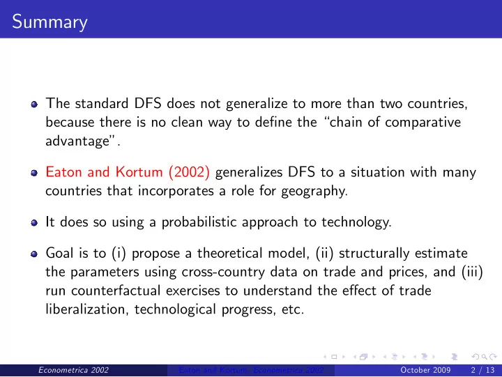
  1. Summary The standard DFS does not generalize to more than two countries, because there is no clean way to de…ne the “chain of comparative advantage”. Eaton and Kortum (2002) generalizes DFS to a situation with many countries that incorporates a role for geography. It does so using a probabilistic approach to technology. Goal is to (i) propose a theoretical model, (ii) structurally estimate the parameters using cross-country data on trade and prices, and (iii) run counterfactual exercises to understand the e¤ect of trade liberalization, technological progress, etc. Econometrica 2002 Eaton and Kortum, Econometrica 2002 () October 2009 2 / 13

  2. Basic setup Continuum of goods j located on unit interval [0,1]. N countries indexed by i . Input cost (labor + intermediates) in country i denoted by c i . Goods are homogeneous and there is perfect competition. E¢ciency of country i in producing good j is z i ( j ) . Cost of producing a unit of good j in country i is c i / z i ( j ) . Econometrica 2002 Eaton and Kortum, Econometrica 2002 () October 2009 3 / 13

  3. Basic setup Geographic barriers are of the iceberg form. To deliver 1 unit from country i to country j requires shipping d ni > 1 units. The price of a good j produced in country i and bought in country j is p ni ( j ) = ( c i z i ( j )) d ni (1) Actual price paid by consumers in country n for good j (after shopping around) is p n ( j ) = min f p ni ( j ) ; i = 1 , ..., N g (2) Preferences are Cobb-Douglas Z 1 0 Q ( j ) ( σ � 1 ) / σ dj ] σ / ( σ � 1 ) U = [ (3) Econometrica 2002 Eaton and Kortum, Econometrica 2002 () October 2009 4 / 13

  4. Technology The e¢ciency of country i in the production of good j is the realization of a random variable, Z i , drawn from a Fréchet distribution F i ( z ) = Pr [ Z i � z ] = e � T i z � θ (4) where T i > 0 and θ > 1. Two parameters: T i is country-speci…c and determines absolute advantage (higher T i implies greater absolute advantage); and θ , common to all countries, determines the variation within the distribution, and thus the scope of comparative advantage. Econometrica 2002 Eaton and Kortum, Econometrica 2002 () October 2009 5 / 13

  5. Prices Since the productivity to produce good j in country i is the realization of a random variable, the price at which i o¤er good j in country n is also the realization of a random variable, c i d ni / Z i . This implies that each country i presents country n with a price distribution, G ni ( p ) = Pr [ P ni � p ] . The probability that P ni � p is the same as the probability that c i d ni / Z i is less than p , which is the same as the probability that Z i is more than c i d ni / p . This implies that G ni ( p ) = Pr [ P ni � p ] = 1 � F i ( c i d ni / p ) (5) Econometrica 2002 Eaton and Kortum, Econometrica 2002 () October 2009 6 / 13

  6. Prices The actual price distribution in country n is then: G n ( p ) = Pr [ P n � p ] = 1 � Π N i ( 1 � G ni ( p )) (6) i.e., 1 minus the probability that the price from all source countries is greater than p . By substituting (5) into (6) we can re-write this expression as N G n ( p ) = 1 � e � Φ n p θ T i ( c i d ni ) � θ ∑ where Φ n = (7) i = 1 It can be shown that trading with more countries or technological improvement lowers prices, whereas greater geographical barriers increases prices. Econometrica 2002 Eaton and Kortum, Econometrica 2002 () October 2009 7 / 13

  7. Properties of price distributions Property (a) The probability of country i providing a good at the lowest price to country n is π ni = ( T i ( c i d ni ) � θ ) / Φ n (8) Because of law of large numbers, π ni is also the fraction of goods i sells in n . Property (b) The price of a good that country n actually buys from any country i also has the distribution G n ( p ) . That is, the price distribution of the goods sold by country i to country n is independent of i . Countries with better access or better technology sell a wider range of goods (increase in the extensive margin), such that the distribution of the prices of what it sells in country n is the same as the overall price distribution in country n . Econometrica 2002 Eaton and Kortum, Econometrica 2002 () October 2009 8 / 13

  8. Properties of price distributions Property (c) The price index for the CES utility function can be shown to be where γ = [ Γ ( θ + 1 � σ p n = γ Φ � 1 / θ )] 1 / ( 1 � σ ) (9) n θ where Γ is the Gamma function. Econometrica 2002 Eaton and Kortum, Econometrica 2002 () October 2009 9 / 13

  9. Trade ‡ows and gravity Property (b) implies that country n ’s average expenditure per good does not vary by source country, so that the fraction of goods country n buys from country i is also the fraction of its expenditure on goods from i : = T i ( c i d ni ) � θ T i ( c i d ni ) � θ π ni = X ni = (10) ∑ N X n Φ n k = 1 T k ( c k d nk ) � θ This is similar to a standard gravity equation: value of exports from i to n depends positively on total expenditure of n and negatively on geographic barriers. Econometrica 2002 Eaton and Kortum, Econometrica 2002 () October 2009 10 / 13

  10. Trade ‡ows and gravity Country i ’s total exports are: d � θ N N mi X m X mi = T i c � θ ∑ ∑ Q i = (11) i Φ m m = 1 m = 1 Combining (10) and (11) gives us ( d ni p n ) � θ X n X ni = Q i (12) ∑ N m = 1 ( d mi p m ) � θ X m Hence, exports from i to n depend on (i) total expenditure of n , X n ; (ii) total sales of exporter, Q i ; and (iii) geographic barriers. Numerator ( ( d ni p n ) � θ X n ) can be interpreted as the market size of destination n as perceived by exporter i , whereas the denominator ( ∑ N m = 1 ( d mi p m ) � θ X m ) can be interpreted as the total world market as perceived by exporter i . Econometrica 2002 Eaton and Kortum, Econometrica 2002 () October 2009 11 / 13

  11. Closing the model To close model, we need to determine c i , which has been taken as given until now. Income of inputs (labor+intermediates) must equal spending by inputs (labor+intermediates). See paper for further details. Econometrica 2002 Eaton and Kortum, Econometrica 2002 () October 2009 12 / 13

  12. Parameter estimates and counterfactuals Use data on 19 OECD countries to estimate parameter values. Run counterfactuals. Example: quantify e¤ects of declining geographic barriers. Example: quantify e¤ect of technological progress in one country on welfare in others. Econometrica 2002 Eaton and Kortum, Econometrica 2002 () October 2009 13 / 13

Download Presentation
Download Policy: The content available on the website is offered to you 'AS IS' for your personal information and use only. It cannot be commercialized, licensed, or distributed on other websites without prior consent from the author. To download a presentation, simply click this link. If you encounter any difficulties during the download process, it's possible that the publisher has removed the file from their server.

Recommend


More recommend