
SLIDE 1
CEE 680 Lecture #30 3/23/2020 1
Lecture #30 Coordination Chemistry: case studies
(Stumm & Morgan, Chapt.6: pg.305‐319)
Benjamin; Chapter 8.1‐8.6
David Reckhow CEE 680 #30 1
Updated: 23 March 2020
Print version
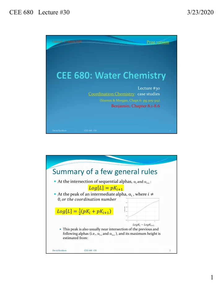
Summary of a few general rules
At the intersection of sequential alphas, i and i+1 : At the peak of an intermediate alpha, i , where 𝑗
0, 𝑝𝑠 𝑢ℎ𝑓 𝑑𝑝𝑝𝑠𝑒𝑗𝑜𝑏𝑢𝑗𝑝𝑜 𝑜𝑣𝑛𝑐𝑓𝑠
This peak is also usually near intersection of the previous and
following alphas (i.e., i‐1 and i+1 ), and its maximum height is estimated from:
David Reckhow CEE 680 #30 2
𝑀𝑝 𝑀 𝑞𝐿 𝑀𝑝 𝑀
𝑞𝐿 𝑞𝐿
LogKx-LogKx+1
- 1
𝑀𝑝𝐿 𝑀𝑝𝐿