
SLIDE 1
Steps to understanding Policy-gradient methods
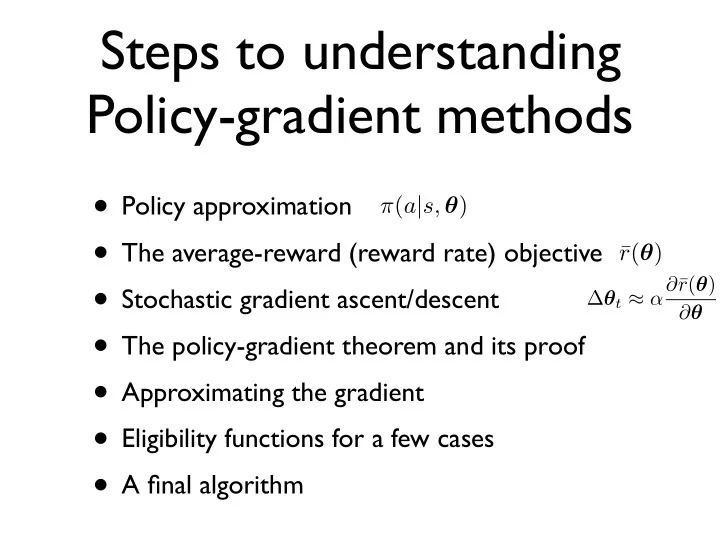
- Policy approximation
- The average-reward (reward rate) objective
- Stochastic gradient ascent/descent
- The policy-gradient theorem and its proof
- Approximating the gradient
- Eligibility functions for a few cases
- A final algorithm
π(a|s, θ)
∆θt ≈ α∂¯ r(θ) ∂θ
¯ r(θ)