Statistical NLP Spring 2011 Lecture 5: Speech Recognition II Dan - PDF document

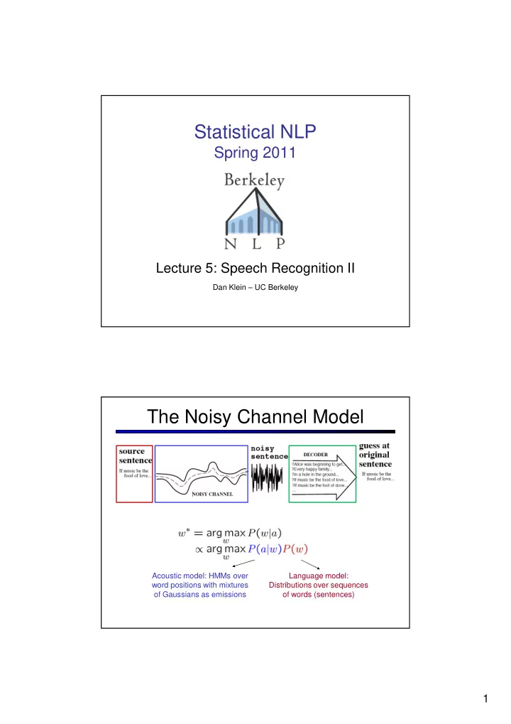
Statistical NLP Spring 2011 Lecture 5: Speech Recognition II Dan Klein – UC Berkeley The Noisy Channel Model Acoustic model: HMMs over Language model: word positions with mixtures Distributions over sequences of Gaussians as emissions of words (sentences) 1

Speech Recognition Architecture Digitizing Speech 2

Frame Extraction � A frame (25 ms wide) extracted every 10 ms 25 ms . . . 10ms a 1 a 2 a 3 Figure from Simon Arnfield Mel Freq. Cepstral Coefficients � Do FFT to get spectral information � Like the spectrogram/spectrum we saw earlier � Apply Mel scaling � Models human ear; more sensitivity in lower freqs � Approx linear below 1kHz, log above, equal samples above and below 1kHz � Plus discrete cosine transform [Graph from Wikipedia] 3

Final Feature Vector � 39 (real) features per 10 ms frame: � 12 MFCC features � 12 delta MFCC features � 12 delta-delta MFCC features � 1 (log) frame energy � 1 delta (log) frame energy � 1 delta-delta (log frame energy) � So each frame is represented by a 39D vector HMMs for Continuous Observations � Before: discrete set of observations � Now: feature vectors are real-valued � Solution 1: discretization � Solution 2: continuous emissions � Gaussians � Multivariate Gaussians � Mixtures of multivariate Gaussians � A state is progressively � Context independent subphone (~3 per phone) � Context dependent phone (triphones) � State tying of CD phone 4

Vector Quantization � Idea: discretization � Map MFCC vectors onto discrete symbols � Compute probabilities just by counting � This is called vector quantization or VQ � Not used for ASR any more; too simple � But: useful to consider as a starting point Gaussian Emissions � VQ is insufficient for real ASR � Hard to cover high- dimensional space with codebook � Moves too much ambiguity from the model to the preprocessing? � Instead: assume the possible values of the observation vectors are normally distributed. � Represent the observation likelihood function as a Gaussian? From bartus.org/akustyk 5

Gaussians for Acoustic Modeling A Gaussian is parameterized by a mean and a variance: � P(x): P(o) is highest here at mean P(o) is low here, far from mean P(x) x Multivariate Gaussians � Instead of a single mean µ and variance σ 2 : � Vector of means µ and covariance matrix Σ � Usually assume diagonal covariance (!) � This isn’t very true for FFT features, but is often OK for MFCC features 6

Gaussians: Size of Σ � µ = [0 0] µ = [0 0] µ = [0 0] � Σ = I Σ = 0.6I Σ = 2I � As Σ becomes larger, Gaussian becomes more spread out; as Σ becomes smaller, Gaussian more compressed Text and figures from Andrew Ng Gaussians: Shape of Σ � As we increase the off diagonal entries, more correlation between value of x and value of y Text and figures from Andrew Ng 7

But we’re not there yet � Single Gaussians may do a bad job of modeling a complex distribution in any dimension � Even worse for diagonal covariances � Solution: mixtures of Gaussians From openlearn.open.ac.uk Mixtures of Gaussians � M mixtures of Gaussians: From robots.ox.ac.uk http://www.itee.uq.edu.au/~comp4702 8

GMMs � Summary: each state has an emission distribution P(x|s) (likelihood function) parameterized by: � M mixture weights � M mean vectors of dimensionality D � Either M covariance matrices of DxD or M Dx1 diagonal variance vectors HMMs for Speech 9

Phones Aren’t Homogeneous 5000 Frequency (Hz) 0 0.48152 ay k 0.937203 Time (s) Need to Use Subphones 10

A Word with Subphones Modeling phonetic context w iy r iy m iy n iy 11

“Need” with triphone models ASR Lexicon: Markov Models 12

Markov Process with Bigrams Figure from Huang et al page 618 Training Mixture Models � Input: wav files with unaligned transcriptions � Forced alignment � Computing the “Viterbi path” over the training data (where the transcription is known) is called “forced alignment” � We know which word string to assign to each observation sequence. � We just don’t know the state sequence. � So we constrain the path to go through the correct words (by using a special example-specific language model) � And otherwise run the Viterbi algorithm � Result: aligned state sequence 13

Lots of Triphones � Possible triphones: 50x50x50=125,000 � How many triphone types actually occur? � 20K word WSJ Task (from Bryan Pellom) � Word internal models: need 14,300 triphones � Cross word models: need 54,400 triphones � Need to generalize models, tie triphones State Tying / Clustering � [Young, Odell, Woodland 1994] � How do we decide which triphones to cluster together? � Use phonetic features (or ‘broad phonetic classes’) � Stop � Nasal � Fricative � Sibilant � Vowel � lateral 14

State Tying � Creating CD phones: � Start with monophone, do EM training � Clone Gaussians into triphones � Build decision tree and cluster Gaussians � Clone and train mixtures (GMMs) � General idea: � Introduce complexity gradually � Interleave constraint with flexibility Standard subphone/mixture HMM Temporal Structure Gaussian Mixtures Model Error rate HMM Baseline 25.1% 15

An Induced Model Standard Model Fully Connected Single Gaussians [Petrov, Pauls, and Klein, 07] Hierarchical Split Training with EM 32.1% 28.7% 25.6% 23.9% HMM Baseline 25.1% 5 Split rounds 21.4% 16

Refinement of the /ih/-phone Refinement of the /ih/-phone 17

�� �� �� �� �� �� � � ae ao ay eh Refinement of the /ih/-phone er ey ih f HMM states per phone r s sil aa ah ix iy z cl k sh n vcl ow l m t v uw aw ax ch w th el dh uh p en oy hh jh ng y b d dx g zh epi 18

Inference � State sequence: Viterbi d 1 -d 6 -d 6 -d 4 -ae 5 -ae 2 -ae 3 -ae 0 -d 2 -d 2 -d 3 -d 7 -d 5 � Phone sequence: Variational d - d - d -d -ae - ae - ae - ae - d - d -d - d - d � Transcription ??? d - ae - d 19