Stable matchings from the perspective of distributed algorithms - - PowerPoint PPT Presentation

Paderborn, 22 October 2009

1 1 2 3 3 2 1 2 1 1 2 2 1 1

YES YES YES NO

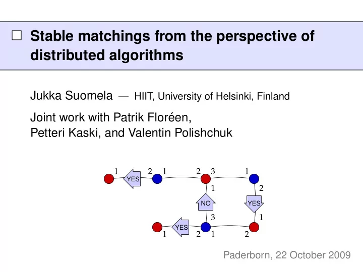
Jukka Suomela — HIIT, University of Helsinki, Finland Joint work with Patrik Floréen, Petteri Kaski, and Valentin Polishchuk

Stable matchings from the perspective of distributed algorithms

1 1 2 3 3 2 1 2 1 1 2 2 1 1

Stable matchings

2 / 45

Part I: Introduction

Input: bipartite graph G = (R ∪ B, E) . . .

• R = red nodes
• B = blue nodes

3 / 45

Stable marriage problem

1 1 2 3 3 2 1 2 1 1 2 2 1 1

Input: bipartite graph G = (R ∪ B, E) and preferences

• 1 = most preferred partner
• but anyone is better than no-one

4 / 45

Stable marriage problem

1 1 2 3 3 2 1 2 1 1 2 2 1 1

Output: a stable matching, i.e., a matching without unstable edges

5 / 45

Stable marriage problem

1 1 2 3 3 2 1 2 1 1 2 2 1 1

Matching: subset M ⊆ E of edges such that each node adjacent to at most one edge in M

6 / 45

Stable marriage problem

1 1 2 3 3 2 1 2 1 1 2 2 1 1

Matching: subset M ⊆ E of edges such that each node adjacent to at most one edge in M

7 / 45

Stable marriage problem

1 1 2 3 3 2 1 2 1 1 2 2 1 1

Matching: subset M ⊆ E of edges such that each node adjacent to at most one edge in M

8 / 45

Stable marriage problem

1 1 2 3 3 2 1 2 1 1 2 2 1 1

Unstable edge: edge {r, b} /

∈ M such that

• r prefers b to r’s current partner (if any)
• b prefers r to b’s current partner (if any)

9 / 45

Stable marriage problem

1 1 2 3 3 2 1 2 1 1 2 2 1 1

Unstable edge: edge {r, b} /

∈ M such that

• r prefers b to r’s current partner (if any)
• b prefers r to b’s current partner (if any)

10 / 45

Stable marriage problem

1 1 2 3 3 2 1 2 1 1 2 2 1 1

Unstable edge: edge {r, b} /

∈ M such that

• r prefers b to r’s current partner (if any)
• b prefers r to b’s current partner (if any)

11 / 45

Stable marriage problem

1 1 2 3 3 2 1 2 1 1 2 2 1 1

No unstable edges =

⇒ stable matching

• Does it always exist?
• How to find one?

12 / 45

Stable marriage problem

1 1 2 3 3 2 1 2 1 1 2 2 1 1

Gale–Shapley

13 / 45

Part II: Finding a stable matching

1 1 2 3 3 2 1 2 1 1 2 2 1 1

An adaptation of the Gale–Shapley algorithm (1962) Begin with an empty matching

14 / 45

Stable marriage problem

1 1 2 3 3 2 1 2 1 1 2 2 1 1 ? ? ? ?

Unmatched red nodes send proposals to their most-preferred neighbours

15 / 45

Stable marriage problem

1 1 2 3 3 2 1 2 1 1 2 2 1 1

YES YES YES NO

Blue nodes accept the best proposal

16 / 45

Stable marriage problem

1 2 3 2 1 2 1 1 2 2 1 1 1 3

Blue nodes accept the best proposal Remove rejected edges and repeat. . .

17 / 45

Stable marriage problem

1 2 3 2 1 2 1 1 2 2 1 1 1 3 ?

Unmatched red nodes send proposals to their most-preferred neighbours

18 / 45

Stable marriage problem

1 2 3 2 1 2 1 1 2 2 1 1 1 3

YES

×

Blue nodes accept the best proposal It is ok to change mind if a better proposal is received!

19 / 45

Stable marriage problem

1 2 3 2 1 1 2 2 1 1 1 3 2 1

Blue nodes accept the best proposal Remove rejected edges and repeat. . .

20 / 45

Stable marriage problem

1 2 3 2 1 1 2 2 1 1 1 3 2 1

Eventually each red node

• is matched, or
• has been rejected by all neighbours

21 / 45

Stable marriage problem

1 2 3 2 1 1 2 2 1 1 1 3 2 1 r b

Let {r, b} /

∈ M: (i) b ∈ B rejected r ∈ R = ⇒ b was matched to a more preferred neighbour = ⇒ {r, b} is not unstable

22 / 45

Stable marriage problem

1 2 3 2 1 1 2 2 1 1 1 3 2 1 r b

Let {r, b} /

∈ M: (ii) r ∈ R did not ask b ∈ B = ⇒ r is matched to a more preferred neighbour = ⇒ {r, b} is not unstable

23 / 45

Stable marriage problem

1 1 2 3 3 2 1 2 1 1 2 2 1 1

The Gale–Shapley algorithm finds a stable matching Ok, that was published 47 years ago, more recent news?

24 / 45

Stable marriage problem

1 1 2 3 3 2 1 2 1 1 2 2 1 1

Stable matchings are unstable

25 / 45

Part III: Stable matchings in a distributed setting

1 1 2 3 3 2 1 2 1 1 2 2 1 1

Node = computer, edge = communication link Efficient distributed algorithms for stable matchings?

26 / 45

Stable matchings in a distributed setting

1 1 2 3 3 2 1 2 1 1 2 2 1 1

YES YES YES NO

The Gale–Shapley algorithm can be interpreted as a distributed algorithm

• proposal, acceptance, rejection: messages

27 / 45

Stable matchings in a distributed setting

1 1 2 3 3 2 1 2 1 1 2 2 1 1

YES YES YES NO

Many nice properties:

• small messages, deterministic
• unique identifiers not needed

28 / 45

Stable matchings in a distributed setting

2 1 1 2 2 1 1 2 2 1 1 2 1 1 1 2 2 1 1 2 2 1 1 2 2 1 1 2 1 1 2 1

But Gale–Shapley isn’t fast – it cannot be fast!

29 / 45

Stable matchings in a distributed setting

2 1 1 2 2 1 1 2 2 1 1 2 1 1 1 2 2 1 1 2 2 1 1 2 2 1 1 2 1 1 2 1

Solution depends on the input in distant parts of network

= ⇒ worst-case running time Ω(diameter)

30 / 45

Stable matchings in a distributed setting

2 1 1 2 2 1 1 2 2 1 1 2 1 1 1 2 2 1 1 2 2 1 1 2 2 1 1 2 1 1 2 1

Stable matchings are unstable! Minor changes in input may require major changes in output

31 / 45

Stable matchings in a distributed setting

Stable matchings are unstable! Minor changes in input may require major changes in output

• This isn’t really what we would expect to happen,

e.g., in real-world large scale social networks

• Very distant parts of the network should not affect

my choices

• Are stable matchings the right problem to study?

Matchings that are more robust and more local?

32 / 45

Stable matchings in a distributed setting

1 1 2 3 3 2 1 2 1 1 2 2 1 1

Truncating Gale–Shapley

33 / 45

Part IV: Almost stable matchings

Our contribution: asking the right questions

• What if we allow a small fraction
• f unstable edges?
• What happens if we run Gale–Shapley

for a small number of rounds? Others have asked similar questions, too. . .

34 / 45

Almost stable matchings

What if we allow a small fraction of unstable edges?

• Biró et al. (2008): finding a maximum matching

with few unstable edges is hard

• Finding any matching with few unstable edges?

Running Gale–Shapley for a small number of rounds?

• Quinn (1985): experimental work suggests

that we get few unstable edges

• Any theoretical guarantees?

35 / 45

Almost stable matchings

Definition: A matching M is ǫ-stable if there are at most ǫ|M| unstable edges Main result: There is a distributed algorithm that finds an ǫ-stable matching in O(∆2/ǫ) rounds Algorithm: Just run the distributed version of Gale–Shapley for that many steps!

∆ = maximum degree of G 36 / 45

Almost stable matchings

1 2 3 2 1 2 1 1 2 2 1 1 1 3

During the Gale–Shapley algorithm:

{r, b} ∈ E is an unstable edge = ⇒ r unmatched and r has not yet proposed b

37 / 45

Almost stable matchings

1 2 3 2 1 2 1 1 2 2 1 1 1 3

Key idea: define total potential

= number of unmatched red nodes with proposals left = how much red nodes could “gain”

if we did not truncate Gale–Shapley

38 / 45

Almost stable matchings

1 1 2 3 3 2 1 2 1 1 2 2 1 1

Key idea: define total potential

= number of unmatched red nodes with proposals left

Initially high

39 / 45

Almost stable matchings

1 2 3 2 1 1 2 2 1 1 1 3 2 1

Key idea: define total potential

= number of unmatched red nodes with proposals left

Zero if we run the full Gale–Shapley

40 / 45

Almost stable matchings

• Potential is non-increasing: if a red node loses

its partner, another red node gains a partner

• Assume that potential is α after round k > 1

= ⇒ α nodes received ‘no’ or ‘break’ in round k = ⇒ at least α edges removed in round k = ⇒ at least (k − 1)α edges removed

in rounds 2, 3, . . . , k

• At most O(∆|M|) edges removed in total

= ⇒ potential O(∆|M|/k) after round k = ⇒ O(∆2|M|/k) unstable edges

41 / 45

Almost stable matchings

Generalises to weighted matchings Applications (in bipartite, bounded-degree graphs):

• Local (2 + ǫ)-approximation algorithm

for maximum-weight matching

• Centralised randomised algorithm for

estimating the size of a stable matching

(All stable matchings have the same size!) 42 / 45

Almost stable matchings

But I think the most interesting observation is this:

• Almost stable matchings are a local problem

(at least in bounded-degree graphs)

• There is a simple local algorithm that finds

a robust, almost stable matching M

• The matching M can be easily maintained

in a dynamic network, constructed by using an efficient self-stabilising algorithm, etc.

43 / 45

Almost stable matchings

1 2 3 2 1 2 1 1 2 2 1 1 1 3

Research question: are almost stable matchings the right concept when we try to understand and analyse real-world social networks, matching markets, etc.?

44 / 45

Almost stable matchings

http://www.cs.helsinki.fi/jukka.suomela/ Stable matching:

• global problem, any solution is unrobust

Almost stable matching:

• local problem, robust solutions exist

No new algorithms needed, just a new analysis

• f the Gale–Shapley algorithm from 1962

45 / 45

Summary