Solving Linear Systems Using Matrices MCV4U: Calculus & Vectors - PDF document

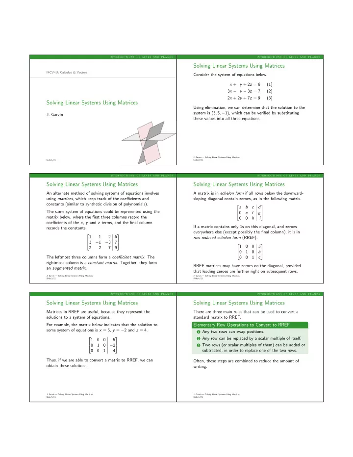
i n t e r s e c t i o n s o f l i n e s a n d p l a n e s i n t e r s e c t i o n s o f l i n e s a n d p l a n e s Solving Linear Systems Using Matrices MCV4U: Calculus & Vectors Consider the system of equations below. x + y + 2 z = 6 (1) 3 x − y − 3 z = 7 (2) 2 x + 2 y + 7 z = 9 (3) Solving Linear Systems Using Matrices Using elimination, we can determine that the solution to the system is (3 , 5 , − 1), which can be verified by substituting J. Garvin these values into all three equations. J. Garvin — Solving Linear Systems Using Matrices Slide 1/21 Slide 2/21 i n t e r s e c t i o n s o f l i n e s a n d p l a n e s i n t e r s e c t i o n s o f l i n e s a n d p l a n e s Solving Linear Systems Using Matrices Solving Linear Systems Using Matrices An alternate method of solving systems of equations involves A matrix is in echelon form if all rows below the downward- using matrices , which keep track of the coefficients and sloping diagonal contain zeroes, as in the following matrix. constants (similar to synthetic division of polynomials).   a b c d The same system of equations could be represented using the 0 e f g   matrix below, where the first three columns record the 0 0 h i coefficients of the x , y and z terms, and the final column If a matrix contains only 1s on this diagonal, and zeroes records the constants. everywhere else (except possibly the final column), it is in  1 1 2 6  row-reduced echelon form (RREF). 3 − 1 − 3 7    1 0 0 a  2 2 7 9 0 1 0 b   The leftmost three columns form a coefficient matrix . The 0 0 1 c rightmost column is a constant matrix . Together, they form RREF matrices may have zeroes on the diagonal, provided an augmented matrix . that leading zeroes are further right on subsequent rows. J. Garvin — Solving Linear Systems Using Matrices J. Garvin — Solving Linear Systems Using Matrices Slide 3/21 Slide 4/21 i n t e r s e c t i o n s o f l i n e s a n d p l a n e s i n t e r s e c t i o n s o f l i n e s a n d p l a n e s Solving Linear Systems Using Matrices Solving Linear Systems Using Matrices Matrices in RREF are useful, because they represent the There are three main rules that can be used to convert a solutions to a system of equations. standard matrix to RREF. For example, the matrix below indicates that the solution to Elementary Row Operations to Convert to RREF some system of equations is x = 5, y = − 2 and z = 4. 1 Any two rows can swap positions. 2 Any row can be replaced by a scalar multiple of itself.  1 0 0 5  0 1 0 − 2 3 Two rows (or scalar multiples of them) can be added or   0 0 1 4 subtracted, in order to replace one of the two rows. Thus, if we are able to convert a matrix to RREF, we can Often, these steps are combined to reduce the amount of obtain these solutions. writing. J. Garvin — Solving Linear Systems Using Matrices J. Garvin — Solving Linear Systems Using Matrices Slide 5/21 Slide 6/21

i n t e r s e c t i o n s o f l i n e s a n d p l a n e s i n t e r s e c t i o n s o f l i n e s a n d p l a n e s Solving Linear Systems Using Matrices Solving Linear Systems Using Matrices Example Next, use elementary row operations to force leading zeroes in rows 2 and 3 (R2 and R3). Specifically, we replace R2 with Solve the linear system R2-3(R1), and R3 with R3-2(R1). x + y + 2 z = 6 (1)  1 1 2 6   1 1 2 6  3 x − y − 3 z = 7 (2) 3 − 1 − 3 7  → 0 − 4 − 9 − 11    2 x + 2 y + 7 z = 9 (3) 2 2 7 9 0 0 3 − 3 The matrix is in echelon form, but has not yet been reduced. First, convert the linear system to an augmented matrix, as We can multiply R3 by 1 3 to solve for z . we did earlier.  1 1 2 6  3 − 1 − 3 7  1 1 2 6   1 1 2 6    2 2 7 9 0 − 4 − 9 − 11  → 0 − 4 − 9 − 11    0 0 3 − 3 0 0 1 − 1 Therefore, z = − 1 is part of the solution. J. Garvin — Solving Linear Systems Using Matrices J. Garvin — Solving Linear Systems Using Matrices Slide 7/21 Slide 8/21 i n t e r s e c t i o n s o f l i n e s a n d p l a n e s i n t e r s e c t i o n s o f l i n e s a n d p l a n e s Solving Linear Systems Using Matrices Solving Linear Systems Using Matrices We still need to convert the 1 and 2 in R1, and the − 9 in The matrix is nearly in RREF. All that remains is to multiply R1 by 1 4 and R2 by − 1 R2, to zeroes to express the matrix in RREF. Start with the 4 . entry in R1C2 by replacing R1 with 4(R1)+R2.  4 0 0 12   1 0 0 3      1 1 2 6 4 0 − 1 13 0 − 4 0 − 20  → 0 1 0 5    0 − 4 − 9 − 11 0 − 4 − 9 − 11  → 0 0 1 − 1 0 0 1 − 1    0 0 1 − 1 0 0 1 − 1 Therefore, we can confirm that the solution to the system of Now “zero-out” the − 1 and − 9 in C3 by replacing R1 with equations is x = 3, y = 5 and z = − 1, or (3 , 5 , − 1). R1+R3, and R2 with R2+9(R3).     4 0 − 1 13 4 0 0 12 0 − 4 − 9 − 11 0 − 4 0 − 20  →    0 0 1 − 1 0 0 1 − 1 J. Garvin — Solving Linear Systems Using Matrices J. Garvin — Solving Linear Systems Using Matrices Slide 9/21 Slide 10/21 i n t e r s e c t i o n s o f l i n e s a n d p l a n e s i n t e r s e c t i o n s o f l i n e s a n d p l a n e s Solving Linear Systems Using Matrices Solving Linear Systems Using Matrices Example Note that the first equation has a coefficient of 0 for x . We can swap R1 and R2, so that the leading zero appears in the Solve the linear system second row instead. 2 y + 3 z = 7 (1)  0 2 3 7   1 2 − 4 − 1  x + 2 y − 4 z = − 1 (2) 1 2 − 4 − 1  → 0 2 3 7    5 x − 2 y + 2 z = − 7 (3) 5 − 2 2 − 7 5 − 2 2 − 7 Zero out the 5 in R3 by replacing R3 with R3-5(R1). In an augmented matrix form, the system of equations is  1 2 − 4 − 1   1 2 − 4 − 1   0 2 3 7  0 2 3 7  → 0 2 3 7 1 2 − 4 − 1      5 − 2 2 − 7 0 − 12 22 − 2 5 − 2 2 − 7 J. Garvin — Solving Linear Systems Using Matrices J. Garvin — Solving Linear Systems Using Matrices Slide 11/21 Slide 12/21

i n t e r s e c t i o n s o f l i n e s a n d p l a n e s i n t e r s e c t i o n s o f l i n e s a n d p l a n e s Solving Linear Systems Using Matrices Solving Linear Systems Using Matrices Zero out the two entries in column 2 by replacing R1 with Zero out the two entries in column 3 by replacing R1 with R1-R2, and R3 with R3+6(R2). R1+7(R3), and R2 with R2-3(R3).  1 2 − 4 − 1   1 0 − 7 − 8   1 0 − 7 − 8   1 0 0 − 1  0 2 3 7 0 2 3 7 0 2 3 7 0 2 0 4  →  →       0 − 12 22 − 2 0 0 40 40 0 0 1 1 0 0 1 1 1 Multiply R2 by 1 Simplify R3 by multiplying by 40 . 2 to put it in RREF.  1 0 − 7 − 8   1 0 − 7 − 8   1 0 0 − 1   1 0 0 − 1  0 2 3 7  → 0 2 3 7 0 2 0 4  → 0 1 0 2       0 0 40 40 0 0 1 1 0 0 1 1 0 0 1 1 Therefore, z = 1. Therefore, the solution to the system is ( − 1 , 2 , 1). J. Garvin — Solving Linear Systems Using Matrices J. Garvin — Solving Linear Systems Using Matrices Slide 13/21 Slide 14/21 i n t e r s e c t i o n s o f l i n e s a n d p l a n e s i n t e r s e c t i o n s o f l i n e s a n d p l a n e s Solving Linear Systems Using Matrices Solving Linear Systems Using Matrices Example Start by replacing R2 with R1-R2, and R3 with R1-R3. Show that the linear system below is inconsistent.     1 1 1 5 1 1 1 5 1 − 2 − 4 8  → 0 3 5 − 3 x + y + z = 5 (1)    1 7 11 3 0 − 6 − 10 2 1 x − 2 y − 4 z = 8 (2) x + 7 y + 11 z = 3 (3) Reduce R3 by multiplying by − 1 2 .  1 1 1 5   1 1 1 5  As always, convert the linear system to an augmented matrix. 0 3 5 − 3  → 0 3 5 − 3      1 1 1 5 0 − 6 − 10 2 0 3 5 − 1 1 − 2 − 4 8   Since R2 and R3 have the same coefficients, but different 1 7 11 3 constants, the system can have no solutions and is inconsistent. J. Garvin — Solving Linear Systems Using Matrices J. Garvin — Solving Linear Systems Using Matrices Slide 15/21 Slide 16/21 i n t e r s e c t i o n s o f l i n e s a n d p l a n e s i n t e r s e c t i o n s o f l i n e s a n d p l a n e s Solving Linear Systems Using Matrices Solving Linear Systems Using Matrices To demonstrate the inconsistency another way, replace R3 Example with R3-R2. Show that the linear system below has infinitely many solutions.  1 1 1 5   1 1 1 5  x + y + z = 5 (1) 0 3 5 − 3 0 3 5 − 3  →    1 x + 3 y − 5 z = 1 (2) 0 3 5 − 1 0 0 0 2 x − 2 y + 10 z = 11 (3) The last line states that 0 x + 0 y + 0 z = 2, which is impossible for any real values of x , y and z . Therefore, the Again, convert the linear system to an augmented matrix. system of equations is inconsistent.  1 1 1 5  1 3 − 5 1   1 − 2 10 11 J. Garvin — Solving Linear Systems Using Matrices J. Garvin — Solving Linear Systems Using Matrices Slide 17/21 Slide 18/21