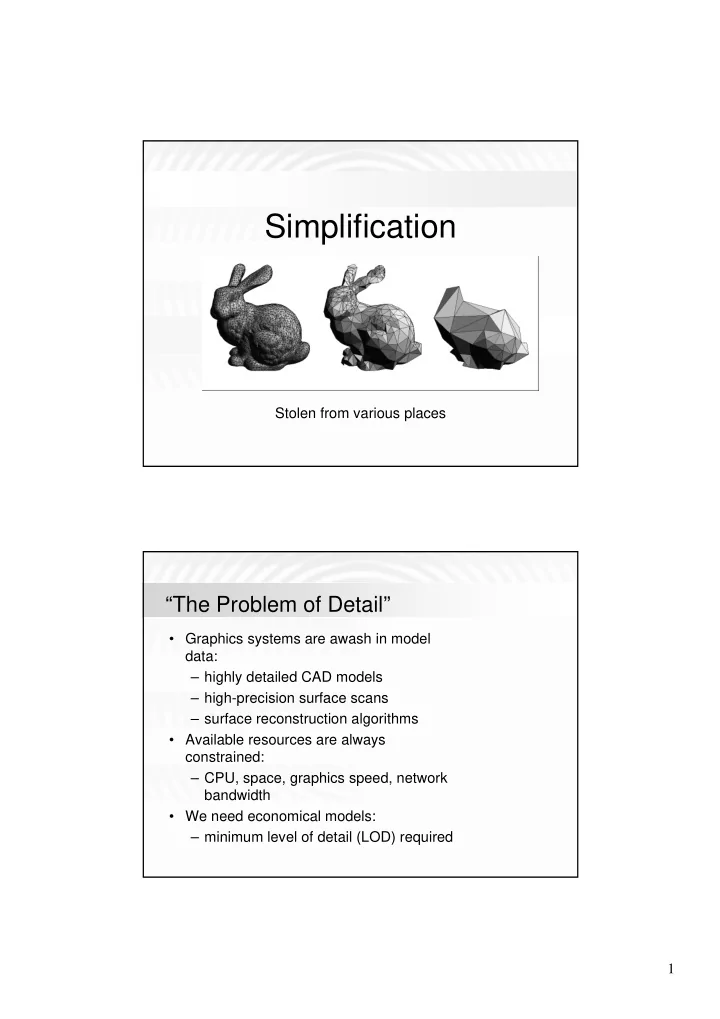
Simplification Stolen from various places The Problem of Detail - - PDF document

1

Simplification

Stolen from various places

“The Problem of Detail”

• Graphics systems are awash in model

data: – highly detailed CAD models – high-precision surface scans – surface reconstruction algorithms

• Available resources are always

constrained: – CPU, space, graphics speed, network bandwidth

• We need economical models:

– minimum level of detail (LOD) required

2

Non-Economical Model

• Motivation

Simplification is an active field of research in various domains: – Cartography: large scale maps generalization – Computer vision: large range data processing – Computer graphics: real time rendering, compression, progressive transmission We focus on polygonal (triangular) surface simplification

3

Single Resolution is Not Enough

– Models used in variety of contexts – Context dictates required detail LOD should vary with context – Context changes dynamically – With what level of coherence?

• generally high coherence in

view

Surface Simplification

4

Triangular meshes

• Common:

– widely supported in hardware – near-universal support in software packages – output of most scanning systems – pragmatic

• Flexible
• Switching representations:

– many applications to convert to and from triangular mesh surface

Surface Simplification Goal

Goal: produce approximations with fewer triangles: – should be as similar as possible to original – computationally efficient process Need criteria for assessing model similarity (some error metric): – similarity of appearance: for display is the ultimate goal – similarity of shape:

• generally easier to compute
• lends itself to more applications other than display

5

Simplification Criteria

Size in scene Complexity: – Geometric (curvature etc.) – Attributes (color, derivatives) Distance Screen size Visibility/Illumination Transmission time View-independent Off-line View-dependent On-line We would like to use models that can change their complexity and adapt according to different parameters.

Distance & Resolution

Distance Resolution

6

Point of View Illumination & Silhouette

Low resolution Adaptive resolution

7

Color Attributes Transmission…

8

Constrained Multiresolution Models

• Encode wide range of levels of detail

– extract appropriate approximations

• can be generated via simplification process

– must have low overhead

• space consumed by representation
• cost of changing level of detail while rendering

– must support the reconstruction of a wide range of levels of details to accommodate a wide range of viewing contexts

• Image pyramids (mip-maps) a good example

– very successful technique for raster images

9

Discrete Multiresolution Models

• Given a model, build a discrete set of approximations

(offline) – can be produced by any simplification system – at run time, simply select which to render using a threshold parameter

• Inter-frame switching causes “popping”

– smooth transition with image blending (cross-disolve) – use geometry blending: geomorphing [Hoppe]

• Supported by several software packages: RenderMan,

Open Inventor, IRIS Performer, ...

10

Limits of Discrete Models

• We may need varying LOD over surface

– E.g.: large surface, oblique view (e.g. on terrain)

• need high detail near the viewer
• need less detail far away

– single LOD will be inappropriate

• either excessively detailed in the distance

(wasteful)

• or insufficiently detailed near viewer (visual

artifacts)

• Doesn’t really exploit available coherence

– small view change may cause large model change

Visualization of Terrains Made Easy

79,382 triangles 25,100 triangles

11

Simplification

Bottom up Top Down

Optimal Approximations

Goal:

• Achieve given error with minimal number of triangles
• Achieve given number of triangles with minimal error

Computationally feasible for curves – O(n) for functions of one variable – but O(n2 log n) for plane curves Intractable for surfaces – NP-hard to find optimal height field [Agarwal–Suri 94] – must also be the case for manifold surfaces

12

Level of Details (LOD)

Each model is in fact a set of models in different level of details. LOD usually means a discrete set of different models:

Decimation primitives

Concentrate locally on part of the mesh and reduce its complexity by a decimation operation (primitive): – Involve near neighbors. Only a small patch of the mesh is affected in each operation – Each operation introduces error – Apply operation which introduces the least error – Incremental

13

Vertex Removal

• Starting with original model, iteratively:

– rank vertices according to their importance – select unimportant vertex, remove it, and its edges. – retriangulate hole

• Remaining vertices are subset of the original set
• A fairly common technique
• Schroeder et al, Soucy et al., Klein et al.

Edge Contraction (Edge Collapse)

• Edge Contraction: two vertices are replaced with one new

vertex removing one edge and two triangles.

• General edge contraction (v1,v2) v’ is performed by

– moving v1 and v2 to position v’ – replacing all occurrences of v2 with v1 – removing v2 and all degenerate triangles

14

Half Edge Contraction

Issue: where should we put the new vertex when contracting? Solution: just use one of the two vertices and remove

• nly one neighbor.

Edge Contraction

Starting with the original model, iteratively – rank all edges with some cost metric – contract minimum cost edge – update edge costs Currently the most popular technique – Hoppe, Garland–Heckbert, Lindstrom-Turk, Ronfard- Rossignac, Guéziec, and several others – simpler than vertex removal (no re-triangulation) – well-defined on any mesh

15

Vertex Pair Contraction

Can also easily contract any pair of vertices – fundamental operation is exactly the same – joins previously unconnected areas – can be used to achieve topological simplification

Contraction Operators Summary

• Edge collapse (v v-1, f f-

2)

• Triangle collapse (vv-2, f f-

4)

• Vertex pair contraction
• Vertex cluster contraction (set
• f vertices)

We want slow simplification!

16

Outline of Decimation Algorithm

While (object not coarse enough) choose best decimation apply to object How do we measure coarseness? How do we choose priority?

Error Metrics for Contraction

Used to sort edges during simplification – reflects amount of geometric error introduced – main differentiating feature among algorithms Must address two interrelated problems – what is the best contraction to perform? – what is the best position v’ for remaining vertex?

• can just choose one of the endpoints
• but can often do better by optimizing position of v’

17

Error Metrics

Define shape distance by:

• Sum
• Max
• Norm L2, L
• Hausdorff Distance

Error computation

Geometric error: – Position difference (vertices triangles) – Volume difference Attribute errors: – Normal difference – Color or function values difference Error calculation or estimation?

18

Error Computation (2)

Local error: Compare the new patch with the previous iteration. + Fast + Memory-less – Accumulates error Global error: Compare the new patch with the original mesh. + Better quality control – Slow – Must remember the original mesh throughout the algorithm

Simplification Error Metrics

Measures:

• Edge length
• Distance to plane
• Curvature
• Volume
• Quadric error metrics

[Garland–Heckbert]

19

Example: Contraction & “Planes” in 2D

Lines defined by neighboring segments – Determine position of new vertex – Accumulate lines for ever larger areas

Original

• After 1 Step
• After 2

Steps

• Measuring Error with Infinite Planes

Why base error on planes? – Faster, but less accurate than distance-to-face – Simple linear system for minimum-error position – Drawback: unlike surface, planes are infinite Related error metrics – Ronfard & Rossignac — max vs. sum – Lindstrom & Turk — similar form; volume-based

20

Quadric Error

• Each vertex has a (conceptual) set of planes

– Error sum of squared distances to planes in set

• Initialize with planes of incident faces

– Consequently, all initial errors are 0

• When contracting pair, use plane set union

– planes(v’) = planes(v1) planes(v2)

• i

i i i i i i T i

d z c y b x a d v n v Error

2 2

) (

Measuring squared distance to the plane is equivalent to:

Quadric Error

Given a plane, we can define a quadric

T T

• T

21

Quadric Error

• 2

2 2

( ) 2 ( ) 2( )

T T T T T T T T T

Q v n v d v n d n v d v nn v dn v d v nn v dn v d

• x

+ v n d x + n v d = x + n v 2d x v n x v n x +d2

The Quadric Error Metric

Sum of quadrics represents set of planes Each vertex has one associated quadric – Error(vi) = i (vi) – Sum quadrics when contracting (vi, vj) v’ – Cost of contraction is (v’) – Exclude duplicate planes from the sum

T

22

The Quadric Error Metric

Sum of endpoint quadrics determines v’ – Optimal placement: choose v’ minimizing (v’) – Fixed placement: select v1 or v2 – Fixed placement is faster but lower quality – It also gives smaller progressive meshes – Fallback to fixed placement if is non-invertible

• Visualizing Quadrics in 3-D

Quadric isosurfaces – Are ellipsoids (maybe degenerate) – Centered around vertices – Characterize shape – Stretch in least- curved directions

23

Sample Model: Dental Mold

• Sample Model: Dental Mold

24

Sample Model: Dental Mold

• Simplification Summary

Spectrum of effective methods developed – high quality; very slow [Hoppe et al, Hoppe] – good quality; varying speed

[Schroeder et al; Klein et al; Ciampalini et al; Guéziec Garland-Heckbert; Ronfard-Rossignac; Lindstrom-Turk]

– lower quality; very fast [Rossignac–Borrel; Low–Tan] Various other differentiating factors: – is topology simplified ? – restricted to manifolds?

25

• Progressive Transmission

Base mesh (M0) is transmitted first. Refinement (e.g. vsplit) records are transmitted later and the mesh reconstructed progressively.

Progressive Meshes

Q: How do we use the model for creating different level of details? A: Multi-resolution model: store the coarsest level object and the encoding of all the decimation operations. Decimation operations order: {d0,d1,d2,…} Each di defines: edge contraction Mi Mi+1 But can also define: vertex split Mi Mi+1 di d-1

i

26

Model Traversal (view independent)

Coarsening – Order: d i+1,di+2,… – History: d0, d1, d2, …,di, Refinement – Order: d i+1,di+2,… – History: d0, d1, d2, …,di, Problems:

• No flexibility in order of operations!
• No adaptiveness in level of details!

A solution should be able to apply coarsening and refinement not necessarily in the order they were produced!

View-Dependent Refinement

Problem: While rendering, there are always faces, which are hidden or far from the viewpoint. Using traditional simplification techniques, those faces are rendered in the same LOD as the complete mesh.

27

cont’

Goal: To generate a progressive representation of a mesh, in which only some of its faces are simplified and the rest are fully detailed.

Vertex split and edge collapse

28

• By combining the PM presentation with the Parent-Child

relationship, a Parent-Child forest can be generated. The root vertices of the forest are M0, which is the most simplified mesh. The leaves of the forest are Mn, which is the original mesh. A cut is defined as a set of edges with the following properties: – Every path from the roots to the leaves is intersected. – Every path is intersected only once.

29

Selective Refinement

• Tree encodes dependency
• f contractions
• Given a vertex hierarchy

forest, a selective refinement mesh can be generated by using selective, out-of-order vsplits and ecols

• perations.
• The current

refined/simplified mesh is a vertex front in the forest.

30

Legal Operations

A face or a vertex are called “Active” if they exist in the current front. Legal vertex split:

• Vs is an active vertex
• The faces {fn0,fn1,fn2,fn3} are all active

Legal edge collapse:

• Vt and Vu are both active
• The faces {fn0,fn1,fn2,fn3} are all active

31

• Applications Beyond Display

Other important applications are appearing – surface editing [Guskov et al 99] – surface morphing [Lee et al 99] – hierarchical bounding volumes – object matching – shape analysis / feature extraction

32

Multiresolution Model Summary

Representations are available to support – progressive transmission – view-dependent refinement – hierarchical computation But limitations remain – vertex hierarchies may over-constrain adaptation – adaptation overhead not suitable for all cases

Looking Ahead

We’ve reached a performance plateau – broad range of methods for certain situations – incremental improvement of existing methods Major progress may require new techniques – broader applicability of simplification – higher quality approximations Needs better understanding of performance – how well, in general, does an algorithm perform?

33

Greater Generality

Model types have complexity issues – tetrahedral volumes, spline patch surfaces, ... Need to handle extremely large data sets – precise scans on the order of 109 triangles – this is where simplification is needed the most – even at 106 triangles, many algorithms fail

Too Large for Many Methods

34

Really Too Large …

• Better Topological Simplification

Imperceptible holes & gaps can be removed – most methods do this only implicitly Few if any methods provide good control – when exactly are holes removed? – will holes above a certain size be preserved? Requires better understanding of the model – when to simplify geometry vs. topology – seems to benefit from more volumetric approach

35

Better Performance Analysis

Better criteria for evaluating similarity – image-based metric more appropriate for display – metrics which accurately account for attributes Most analysis has been case-based – measure/compare performance on 1 data set More thorough analysis is required – theoretical analysis of quality [Heckbert-Garland 99] – provably good approximations possible?

Conclusions

Substantial progress since 1992 – simplification of 3D surfaces – multiresolution representations (PM, hierarchies) – application of multiresolution in different areas There remains much room for improvement – more effective, more general simplification – better analysis and understanding of results – other multiresolution representations