Simplex Method The beer problem: we want to produce beer, either - - PowerPoint PPT Presentation

Arthur Charpentier, Master Statistique & Économétrie - Université Rennes 1 - 2017

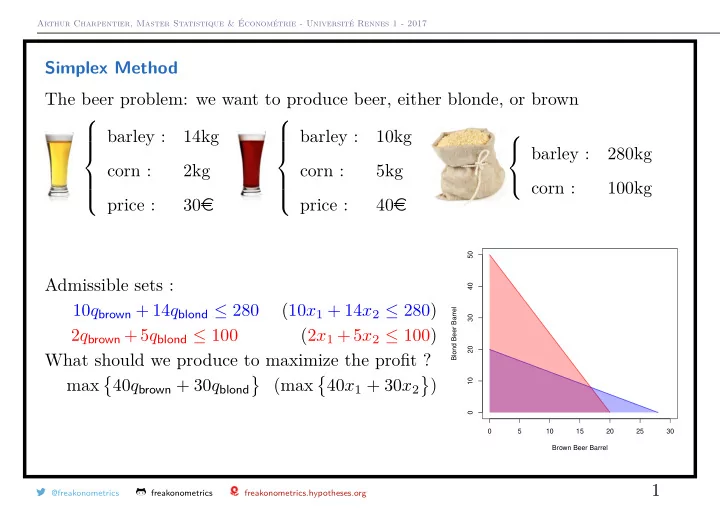
Simplex Method The beer problem: we want to produce beer, either blonde, or brown          barley : 14kg corn : 2kg price : 30e          barley : 10kg corn : 5kg price : 40e    barley : 280kg corn : 100kg Admissible sets : 10qbrown + 14qblond ≤ 280 (10x1 + 14x2 ≤ 280) 2qbrown +5qblond ≤ 100 (2x1 +5x2 ≤ 100) What should we produce to maximize the profit ? max

• 40qbrown + 30qblond
• (max
• 40x1 + 30x2
• )

@freakonometrics freakonometrics freakonometrics.hypotheses.org

1

5 10 15 20 25 30 10 20 30 40 50 Brown Beer Barrel Blond Beer Barrel

Arthur Charpentier, Master Statistique & Économétrie - Université Rennes 1 - 2017

Simplex Method First step: enlarge the space, 10x1 + 14x2 ≤ 280 becomes 10x1 + 14x2 − u1 = 280 (so called slack variables) max

• 40x1 + 30x2
• s.t. 10x1 + 14x2 + u1 = 280

s.t. 2x1 + 5x2 + u2 = 100 s.t. x1, x2, u1, u2 ≥ 0 summarized in the following table, see wikibook x1 x2 u1 u2 (1) 10 14 1 280 (2) 2 5 1 100 max 40 30

@freakonometrics freakonometrics freakonometrics.hypotheses.org

2

Arthur Charpentier, Master Statistique & Économétrie - Université Rennes 1 - 2017

Simplex Method Consider a linear programming problem written in a standard form. min

• cTx
• (1a)

subject to Ax = b , (1b) x ≥ 0 . (1c) Where x ∈ Rn, A is am × n matrix, b ∈ Rm and c ∈ Rn. Assume that rank(A) = m (rows of A are linearly independent) Introduce slack variables to turn inequality constraints into equality constraints with positive unknowns : any inequality a1 x1 + · · · + an xn ≤ c can be replaced by a1 x1 + · · · + an xn + u = c with u ≥ 0. Replace variables which are not sign-constrained by differences : any real number x can be written as the difference of positive numbers x = u − v with u, v ≥ 0.

@freakonometrics freakonometrics freakonometrics.hypotheses.org

3

Arthur Charpentier, Master Statistique & Économétrie - Université Rennes 1 - 2017

Simplex Method Example : maximize {x1 + 2 x2 + 3 x3} subject to x1 + x2 − x3 = 1 , −2 x1 + x2 + 2 x3 ≥ −5 , x1 − x2 ≤ 4 , x2 + x3 ≤ 5 , x1 ≥ 0 , x2 ≥ 0 . minimize {−x1 − 2 x2 − 3 u + 3 v} subject to x1 + x2 − u + v = 1 , 2 x1 − x2 − 2 u + 2 v + s1 = 5 , x1 − x2 + s2 = 4 , x2 + u − v + s3 = 5 , x1, x2, u, v, s1, s2, s3 ≥ 0 .

@freakonometrics freakonometrics freakonometrics.hypotheses.org

4

Arthur Charpentier, Master Statistique & Économétrie - Université Rennes 1 - 2017

Simplex Method Write the coefficients of the problem into a tableau x1 x2 u v s1 s2 s3 1 1 −1 1 1 2 −1 −2 2 1 5 1 −1 1 4 1 1 −1 1 5 −1 −2 −3 3 with constraints on top and coefficients of the objective function are written in a separate bottom row (with a 0 in the right hand column) we need to choose an initial set of basic variables which corresponds to a point in the feasible region of the linear program-ming problem. E.g. x1 and s1, s2, s3

@freakonometrics freakonometrics freakonometrics.hypotheses.org

5

Arthur Charpentier, Master Statistique & Économétrie - Université Rennes 1 - 2017

Simplex Method Use Gaussian elimination to (1) reduce the selected columns to a permutation of the identity matrix (2) eliminate the coefficients of the objective function x1 x2 u v s1 s2 s3 1 1 −1 1 1 −3 1 3 −2 1 −1 1 3 1 1 −1 1 5 −1 −4 4 1 the objective function row has at least one negative entry

@freakonometrics freakonometrics freakonometrics.hypotheses.org

6

Arthur Charpentier, Master Statistique & Économétrie - Université Rennes 1 - 2017

Simplex Method x1 x2 u v s1 s2 s3 1 1 −1 1 1 −3 1 3 −2 1 −1 1 3 1 1 −1 1 5 −1 −4 4 1 This new basic variable is called the entering variable. Correspondingly, one formerly basic variable has then to become nonbasic, this variable is called the leaving variable.

@freakonometrics freakonometrics freakonometrics.hypotheses.org

7

Arthur Charpentier, Master Statistique & Économétrie - Université Rennes 1 - 2017

Simplex Method The entering variable shall correspond to the column which has the most negative entry in the cost function row the most negative cost function coefficient in column 3, thus u shall be the entering variable The leaving variable shall be chosen as follows : Compute for each row the ratio

• f its right hand coefficient to the corresponding coefficient in the entering

variable column. Select the row with the smallest finite positive ratio. The leaving variable is then determined by the column which currently owns the pivot in this row. The smallest positive ratio of right hand column to entering variable column is in row 3, as 3 1 < 5

• 1. The pivot in this row points to s2 as the leaving variable.

@freakonometrics freakonometrics freakonometrics.hypotheses.org

8

Arthur Charpentier, Master Statistique & Économétrie - Université Rennes 1 - 2017

Simplex Method x1 x2 u v s1 s2 s3 1 1 −1 1 1 −3 1 3 −2 1 −1 1 3 1 1 −1 1 5 −1 −4 4 1

@freakonometrics freakonometrics freakonometrics.hypotheses.org

9

Arthur Charpentier, Master Statistique & Économétrie - Université Rennes 1 - 2017

Simplex Method After going through the Gaussian elimination once more, we arrive at x1 x2 u v s1 s2 s3 1 −1 1 4 −3 1 3 −2 1 −1 1 3 3 −1 1 2 −9 4 13 Here x2 will enter and s3 will leave

@freakonometrics freakonometrics freakonometrics.hypotheses.org

10

Arthur Charpentier, Master Statistique & Économétrie - Université Rennes 1 - 2017

Simplex Method After Gaussian elimination, we find x1 x2 u v s1 s2 s3 1

2 3 1 3 14 3

1 −1 1 5 1 −1

1 3 2 3 13 3

1 − 1

3 1 3 2 3

1 3 19 There is no more negative entry in the last row, the cost cannot be lowered

@freakonometrics freakonometrics freakonometrics.hypotheses.org

11

Arthur Charpentier, Master Statistique & Économétrie - Université Rennes 1 - 2017

Simplex Method The algorithm is over, we now have to read off the solution (in the last column) x1 = 14 3 , x2 = 2 3, x3 = u = 13 3 , s1 = 5, v = s2 = s3 = 0 and the minimal value is −19

@freakonometrics freakonometrics freakonometrics.hypotheses.org

12

Arthur Charpentier, Master Statistique & Économétrie - Université Rennes 1 - 2017

Duality Consider a transportation problem. Some good is available at location A (at no cost) and may be transported to locations B, C, and D according to the following directed graph B

4

• 3
• A

2

• 1
• D

C

5

• On each of the edges, the unit cost of transportation is cj for j = 1, . . . , 5.

At each of the vertices, bi units of the good are sold, where i = B, C, D. How can the transport be done most efficiently?

@freakonometrics freakonometrics freakonometrics.hypotheses.org

13

Arthur Charpentier, Master Statistique & Économétrie - Université Rennes 1 - 2017

Duality Let xj denotes the amount of good transported through edge j We have to solve minimize {c1 x1 + · · · + c5 x5} (2) subject to x1 − x3 − x4 = bB , (3) x2 + x3 − x5 = bC , (4) x4 + x5 = bD . (5) Constraints mean here that nothing gets lost at nodes B, C, and D, except what is sold.

@freakonometrics freakonometrics freakonometrics.hypotheses.org

14

Arthur Charpentier, Master Statistique & Économétrie - Université Rennes 1 - 2017

Duality Alternatively, instead of looking at minimizing the cost of transportation, we seek to maximize the income from selling the good. maximize {yB bB + yC bC + yD bD} (6) subject to yB − yA ≤ c1 , (7) yC − yA ≤ c2 , (8) yC − yB ≤ c3 , (9) yD − yB ≤ c4 , (10) yD − yC ≤ c5 . (11) Constraints mean here that the price difference cannot not exceed the cost of transportation.

@freakonometrics freakonometrics freakonometrics.hypotheses.org

15

Arthur Charpentier, Master Statistique & Économétrie - Université Rennes 1 - 2017

Duality Set x =      x1 . . . x5      , y =      yB yC yD      , and A =      1 −1 −1 1 1 −1 1 1      , The first problem - primal problem - is here minimize {cTx} subject to Ax = b, x ≥ 0 . and the second problem - dual problem - is here maximize {yTb} subject to yTA ≤ cT .

@freakonometrics freakonometrics freakonometrics.hypotheses.org

16

Arthur Charpentier, Master Statistique & Économétrie - Université Rennes 1 - 2017

Duality The minimal cost and the maximal income coincide, i.e., the two problems are

• equivalent. More precisely, there is a strong duality theorem

Theorem The primal problem has a nondegenerate solution x if and only if the dual problem has a nondegenerate solution y. And in this case yTb = cTx. See Dantzig & Thapa (1997) Linear Programming

@freakonometrics freakonometrics freakonometrics.hypotheses.org

17