
SLIDE 1
Page 1
Particle Filters++
Pieter Abbeel UC Berkeley EECS
Many slides adapted from Thrun, Burgard and Fox, Probabilistic Robotics
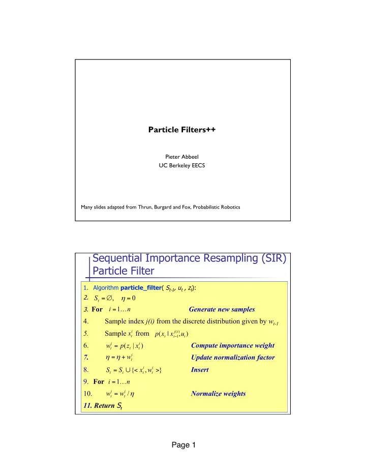
- 1. Algorithm particle_filter( St-1, ut , zt):
2.
- 3. For Generate new samples
4. Sample index j(i) from the discrete distribution given by wt-1 5. Sample from 6. Compute importance weight 7. Update normalization factor 8. Insert
- 9. For
10. Normalize weights
- 11. Return St
, = ∅ = η
t
S n i … 1 = } , { > < ∪ =
i t i t t t
w x S S
i t
w + =η η
i t
x p(xt | x j(i)
t!1,ut)
) | (
i t t i t
x z p w = n i … 1 = η /
i t i t