Sebastian Hack, Christian Hammer, Jan Reineke Saarland University - - PowerPoint PPT Presentation

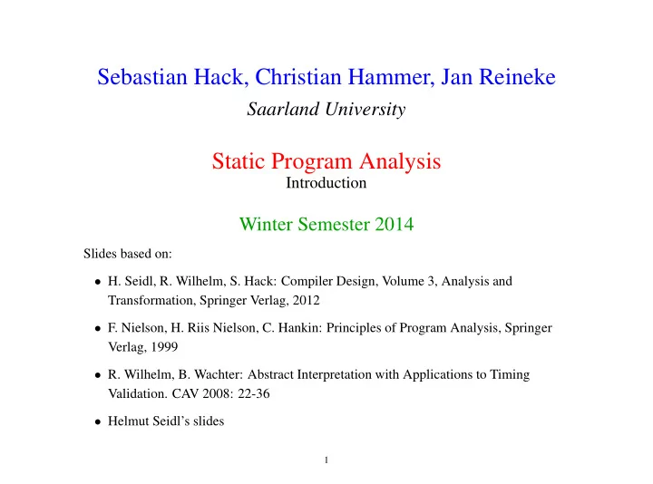
Sebastian Hack, Christian Hammer, Jan Reineke

Saarland University

Static Program Analysis

Introduction

Winter Semester 2014

Slides based on:

• H. Seidl, R. Wilhelm, S. Hack: Compiler Design, Volume 3, Analysis and

Transformation, Springer Verlag, 2012

• F. Nielson, H. Riis Nielson, C. Hankin: Principles of Program Analysis, Springer

Verlag, 1999

• R. Wilhelm, B. Wachter: Abstract Interpretation with Applications to Timing
• Validation. CAV 2008: 22-36
• Helmut Seidl’s slides

1

A Short History of Static Program Analysis

• Early high-level programming languages were implemented on very

small and very slow machines.

• Compilers needed to generate executables that were extremely

efficient in space and time.

• Compiler writers invented efficiency-increasing program

transformations, wrongly called optimizing transformations.

• Transformations must not change the semantics of programs.
• Enabling conditions guaranteed semantics preservation.
• Enabling conditions were checked by static analysis of programs.

2

Theoretical Foundations of Static Program Analysis

• Theoretical foundations for the solution of recursive equations:

Kleene (30s), Tarski (1955)

• Gary Kildall (1972) clarified the lattice-theoretic foundation of

data-flow analysis.

• Patrick Cousot (1974) established the relation to the

programming-language semantics.

3

Static Program Analysis as a Verification Method

• Automatic method to derive invariants about program behavior,

answers questions about program behavior: – will index always be within bounds at program point p? – will memory access at p always hit the cache?

• answers of sound static analysis are correct, but approximate: don’t

know is a valid answer!

• analyses proved correct wrt. language semantics,

4

1

Introduction

a simple imperative programming language with:

• variables

/ / registers

• R = e;

/ / assignments

• R = M[e];

/ / loads

• M[e1] = e2;

/ / stores

• if (e) s1 else s2

/ / conditional branching

• goto L;

/ / no loops An intermediate language into which (almost) everything can be

• translated. In particular, no procedures. So, only intra-procedural

analyses!

5

2

Example — Rules-of-Sign Analysis

Problem: Determine at each program point the sign of the values of all variables of numeric type. Example program: 1: x = 0; 2: y = 1; 3: while (y > 0) do 4: y = y + x; 5: x = x + (-1);

6

Program representation as control-flow graphs

1 2 4 3

y = 1 x = 0 y = y+x

5

x = x+(-1)

true(y>0) false(y>0) 7

We need the following ingredients:

• a set of information elements, each a set of possible signs,
• a partial order, “⊑”, on these elements, specifying the ”relative

strength” of two information elements,

• these together form the abstract domain, a lattice,
• functions describing how signs of variables change by the execution
• f a statement, abstract edge effects,
• these need an abstract arithmetic, an arithmetic on signs.

8

We construct the abstract domain for single variables starting with the lattice Signs = 2{−,0,+} with the relation “⊑” =“⊆”. { } {+} {0,+} {-,0} {-} {-,0,+} {-,+} {0}

9

The analysis should ”bind” program variables to elements in Signs. So, the abstract domain is D = (Vars → Signs)⊥, a Sign-environment. ⊥ ∈ D is the function mapping all arguments to {}. The partial order on D is D1 ⊑ D2 iff D1 = ⊥

• r

D1 x ⊆ D2 x (x ∈ Vars) Intuition? D1 is at least as precise as D2 since D2 admits at least as many signs as D1

10

The analysis should ”bind” program variables to elements in Signs. So, the abstract domain is D = (Vars → Signs)⊥. a Sign-environment. ⊥ ∈ D is the function mapping all arguments to {}. The partial order on D is D1 ⊑ D2 iff D1 = ⊥

• r

D1 x ⊆ D2 x (x ∈ Vars) Intuition? D1 is at least as precise as D2 since D2 admits at least as many signs as D1

11

How did we analyze the program?

1 2 4 3

y = 1 x = 0 y = y+x

5

x = x+(-1)

true(y>0) false(y>0)

In particular, how did we walk the lattice for y at program point 5?

{ } {+} {0,+} {-,0} {-} {-,0,+} {-,+} {0}

12

How is a solution found? Iterating until a fixed-point is reached

1 2 4 3

y = 1 x = 0 y = y+x

5

x = x+(-1)

true(y>0) false(y>0)

1 2 3 4 5 x y x y x y x y x y x y

13

Idea:

• We want to determine the sign of the values of expressions.

14

Idea:

• We want to determine the sign of the values of expressions.
• For some sub-expressions, the analysis may yield

{+, −, 0}, which means, it couldn’t find out.

15

Idea:

• We want to determine the signs of the values of expressions.
• For some sub-expressions, the analysis may yield

{+, −, 0}, which means, it couldn’t find out.

• We replace the concrete operators

✷ working on values by abstract operators ✷♯ working on signs:

16

Idea:

• We want to determine the signs of the values of expressions.
• For some sub-expressions, the analysis may yield

{+, −, 0}, which means, it couldn’t find out.

• We replace the concrete operators

✷ working on values by abstract operators ✷♯ working on signs:

• The abstract operators allow to define an abstract evaluation of

expressions: [ [e] ]♯ : (Vars → Signs) → Signs

17

Determining the sign of expressions in a Sign-environment works as follows: [ [c] ]♯ D =        {+} if c > 0 {−} if c < 0 {0} if c = 0 [ [v] ]♯ = D(v) [ [e1 ✷ e2] ]♯ D = [ [e1] ]♯ D ✷♯ [ [e2] ]♯ D [ [✷e] ]♯ D = ✷♯[ [e] ]♯ D

18

Abstract operators working on signs (Addition) +# {0} {+} {-} {-, 0} {-, +} {0, +} {-, 0, +} {0} {0} {+} {+} {-} {-, 0} {-, +} {0, +} {-, 0, +} {-, 0, +}

19

Abstract operators working on signs (Multiplication) ×# {0} {+} {-} {-, 0} {-, +} {0, +} {-, 0, +} {0} {0} {0} {+} {-} {-, 0} {-, +} {0, +} {-, 0, +} {0} Abstract operators working on signs (unary minus) −# {0} {+} {-} {-, 0} {-, +} {0, +} {-, 0, +} {0} {-} {+} {+, 0} {-, +} {0, -} {-, 0, +}

20

Working an example:

D = {x → {+}, y → {+}} [ [x + 7] ]♯ D = [ [x] ]♯ D +♯ [ [7] ]♯ D = {+} +♯ {+} = {+} [ [x + (−y)] ]♯ D = {+} +♯ (−♯[ [y] ]♯ D ) = {+} +♯ (−♯{+}) = {+} +♯ {−} = {+, −, 0}

21

[ [lab] ]♯ is the abstract edge effects associated with edge k. It depends only on the label lab: [ [;] ]♯ D = D [ [true (e)] ]♯ D = D [ [false (e)] ]♯ D = D [ [x = e;] ]♯ D = D ⊕ {x → [ [e] ]♯ D} [ [x = M[e];] ]♯ D = D ⊕ {x → {+, −, 0}} [ [M[e1] = e2;] ]♯ D = D ... whenever D = ⊥ These edge effects can be composed to the effect of a path π = k1 . . . kr: [ [π] ]♯ = [ [kr] ]♯ ◦ . . . ◦ [ [k1] ]♯

22

Consider a program node v: → For every path π from program entry start to v the analysis should determine for each program variable x the set of all signs that the values of x may have at v as a result of executing π. → Initially at program start, no information about signs is available. → The analysis computes a superset of the set of signs as safe information. = = ⇒ For each node v, we need the set: S[v] =

• {[

[π] ]♯⊥ | π : start →∗ v}

23

Question:

How do we compute S[u] for every program point u?

Idea:

Collect all constraints on the values of S[u] into a system of constraints: S[start] ⊇ ⊥ S[v] ⊇ [ [k] ]♯ (S[u]) k = (u, _, v) edge

24

Question:

How can we compute S[u] for every program point u?

Idea:

Collect all constraints on the values of S[u] into a system of constraints: S[start] ⊇ ⊥ S[v] ⊇ [ [k] ]♯ (S[u]) k = (u, _, v) edge Why ⊇?

25

Wanted:

• a least solution

(why least?)

• an algorithm that computes this solution

Example:

26

1 2 4 3

y = 1 x = 0 y = y+x

5

x = x+(-1)

true(y>0) false(y>0)

S[0] ⊇ ⊥ S[1] ⊇ S[0] ⊕ {x → {0}} S[2] ⊇ S[1] ⊕ {y → {+}} S[2] ⊇ S[5] ⊕ {x → [ [x + (−1)] ]♯ S[5]} S[3] ⊇ S[2] S[4] ⊇ S[2] S[5] ⊇ S[4] ⊕ {y → [ [y + x] ]♯ S[4]}

27