SeaTides Hokkaido North 13 MHz Pacific Ocean Tsugaru Strait - - PowerPoint PPT Presentation

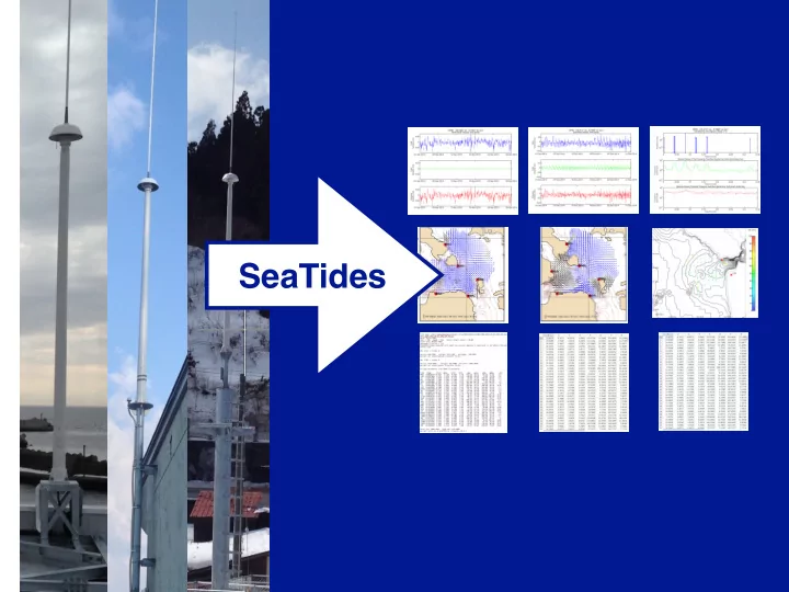
SeaTides

Tsugaru Strait North Pacific Ocean

Honshu Hokkaido

CTD

13 MHz 13 MHz 13 MHz

Vel (cm/s)

total vector
 tuv files

total vector tuv files

t_tide: Publically available tidal anaysis tool

t_tide requirements

http://www.oco.noaa.gov/tideGauges.html

Tide Gauge (generates scalar timeseries

• f water pressure or elevation)

Combined velocity vector data from two or more SeaSondes


• MATLAB or Fortran
• PC or Mac
• Timeseries, scalar or vector

SeaTides requirements

• Compiled SeaTides
• Mac
• Timeseries, tuv files

SeaTides Components

• 1. tuv file conversion
• 2. tidal ellipse
• 3. total, tidal, residual timeseries
• 4. converts tidal and residual timeseries into tuv

SeaTides tuv file conversion

gebco.net ngdc.noaa.gov

gebco.net ngdc.noaa.gov

gebco.net ngdc.noaa.gov

gebco.net ngdc.noaa.gov

• tidal analysis,


at least one month

Velocity Timeseries

gebco.net ngdc.noaa.gov

Velocity Timeseries Velocity Timeseries Velocity Timeseries

3D Timeseries Matrix

removes pages (grid points) with < 50% coverage

Filtered 3D Timeseries Matrix

SeaTides Components

• 1. tuv file conversion
• 2. tidal ellipse
• 3. total, tidal, residual timeseries
• 4. converts tidal and residual timeseries into tuv

gebco.net ngdc.noaa.gov gebco.net ngdc.noaa.gov

SeaTides Tidal Ellipse Plots

maximum major axis = 17 cm/s maximum major axis = 29 cm/s

gebco.net ngdc.noaa.gov

cw ccw cw ccw

• Kyoto University Ocean General 


Circulation Model

• M2 dominant in elevation
• K1 dominant in velocity

gebco.net ngdc.noaa.gov

cw ccw

235

SeaTides Figure Names

East-West (u) North-South (v)

Tidal Velocity (cm/s)

Residual Velocity (cm/s)

Total Velocity (cm/s)

K1 2SK5

tidal spectrum residual spectrum East-West North-South North-South East-West

gebco.net ngdc.noaa.gov

cw ccw

Tidal Velocity (cm/s)

Residual Velocity (cm/s)

Total Velocity (cm/s)

North-South (v) East-West (u)

K1 O1 M2 S2 2MK5

East-West North-South North-South East-West

SeaTides Components

• 1. tuv file conversion
• 2. tidal ellipse
• 3. total, tidal, residual timeseries
• 4. converts total, tidal, and residual timeseries into tuv

gebco.net ngdc.noaa.gov

total vector
 tuv files

Total Signal

Vel (cm/s)

tidal vector
 tuv files

Tidal Signal

Vel (cm/s)

Tidal Signal

residual vector
 tuv files

Residual Signal

Vel (cm/s)

Residual Signal

CTD

28-29 July 2014

Tsugaru Strait North Pacific Ocean

Honshu Hokkaido

CTD

13 MHz 13 MHz 13 MHz

28-29 July 2014 4 m depth 7 m depth 18 m depth

spiciness

Upper Level Depth ~ 4 m

Lines of Constant Density (kg/m3)

Spicy (warm, salty) > 0 Bland (cool, fresh) < 0

< 0

spiciness

Upper Level Depth ~ 4 m

Lines of Constant Density (kg/m3)

Spicy (warm, salty) > 0 Bland (cool, fresh) < 0

< 0

spur of warm water, 33.9 salinity, spiciness ~3 two intrusions of cooler fresher water

spiciness

Upper Level Depth ~ 4 m

Lines of Constant Density (kg/m3)

Middle Level Depth ~ 7 m

Lines of Constant Density (kg/m3)

28-29 July 2014 28-29 July 2014

Lower Level Depth ~ 18 m

spiciness

28-29 July 2014

(TW) Tsugaru Warm Current (S-TW) Tsugaru Warm Current, surface mode (S-OW) Oyashio water system, surface mode

Upper Level Depth ~ 4 m

(S-OW) Oyashio water system, surface mode

28-29 July 2014

Lines of Constant Density (kg/m3)

Temperature (Deg C) Salinity

spiciness

spicy, warm water spur and waters with density > 24 kg/m3 intrusions of cooler fresher water waters in the same salinity band but lower temperature and density

(S-TW) Tsugaru Warm Current, 
 surface mode (TW) Tsugaru Warm Current

Middle Level Depth ~ 7 m

28-29 July 2014

Lines of Constant Density (kg/m3)

spiciness

Temperature (Deg C) Salinity

(S-OW) Oyashio water system, surface mode

spicy, warm water spur and waters with density > 24 kg/m3 intrusions of cooler fresher water waters in the same salinity band but lower temperature and density

(S-TW) Tsugaru Warm Current, 
 surface mode (TW) Tsugaru Warm Current

Lower Level Depth ~ 18 m

28-29 July 2014

Lines of Constant Density (kg/m3)

Temperature (Deg C) Salinity

spiciness

(S-OW) Oyashio water system, surface mode (S-TW) Tsugaru Warm Current, 
 surface mode (TW) Tsugaru Warm Current

Residual Signal

CTD

28-29 July 2014

(TW) Tsugaru Warm Current (S-TW) Tsugaru Warm Current, surface mode (S-OW) Oyashio water system, surface mode

Why tidal analysis?

• Tidal signal strength relative to other signals (if the

tidal signal is significant, then you can predict that component a predicitive tool)

• Understand the mechanism behind features like

upwelling eddies, asociated with biological productivity and fishing grounds, are they driven by tidal forcing, seasonal forcing?

• What other signals are present, removing the tides

might reveal other forcing

SeaTides Conclusion

• Converts large quantities of spatial data into timeseries

format

• Allows visual check on timeseries format
• Provides opportunity to examine tidally driven features

against bathymetry over large areas of ocean

• Provides opportunity to examine non-tidal mechanisms
• SeaTides + SeaDisplay allows movie-making of total,

tidal, and residual data

• A minimum of one month of data is recommended, more

may be run depending on the size of the dataset

Rayleigh Criterion

Constituents separated by at least a complete period over the data length can be identified. To separate M2 and S2: T(M2) = 12.42 hr speed=360/T=360/12.42=28.986 deg/hr T(S2) = 12.00 hr speed=360/T=360/12.00=30.000 deg/hr 360/(30-28.986) = 352.94 hrs = 14.7 days of data needed for O1 and K1: 360/(25.82-23.93) = 7.94 days of data needed

Nyquist Frequency

To quantify a phenomenon of period T, the sample rate may not be greater than T/2. If the period is 12 hours, the sampling rate dt must be < or = 6 hours. If you have a set sampling rate (say dt=2 hours), then only mechanisms with a period twice that or greater can be quantified: T >= 2*dt = 4 hours In terms of frequency, with a sampling frequency, n, of twice a day, or 2/24 = 1/12 hours mechanisms with frequency, N, with frequencies smaller or equal to 1/24 hours can be quantified: N <= 0.5n = 0.5*2/24 = 1/24 hour

snr = [(major axis velocity)/(error)]^2

• snr=[(major axis velocity)/(error)]2
• threshold is set by user
• least squares fit,
• difference between input

velocity and tidally predicted velocity, squares it.

• matrix algebra minimizes

the difference.

• statistical look up tables

determine which are in 95% confidence interval.

Confidence versus Signal to Noise Ratio (snr)

• oyashio
• depth Luu at all study. ADCP measurements at 25 m depth show amplitudes of

K1 and M2 are roughly 0.35 m/s, with max speed of K1 off Cape > 1m/s. model depths not sp’d.

• Tsugaru Strait 128 m depth on average (Luu et al, 2011)
• waters of the East/Japan Sea more saline than the North Pacific waters and are

cold enough to modify propreties in western North Pacific waters (Luu et all, 2011, citing others)

• TWC a throughflow from East/Japan Sea to North Pacific. TWC 1.0 Sv to 2.1 Sv
• southward residual in strait - look at other timeseries. can corliolis be present

here?

• t_tide harominic ana
• tidal ellipses O1, S1, S2 (ellipses over ridge)