Search Space Analysis slightly adapted from slides for SLS:FA, - PDF document

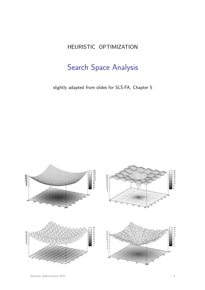
HEURISTIC OPTIMIZATION Search Space Analysis slightly adapted from slides for SLS:FA, Chapter 5 200 24 180 22 160 20 200 24 180 140 18 22 160 120 16 140 20 120 100 14 18 100 80 80 16 12 60 14 40 60 10 20 12 40 8 0 10 20 6 8 0 4 6 4 600 30 400 20 200 10 -600 -30 0 0 -400 -20 -200 -10 -10 -200 0 0 -20 200 -400 10 400 20 30 -30 -600 600 80 18 16 70 14 80 18 60 70 12 16 50 60 14 10 50 40 12 8 40 30 10 30 6 20 20 8 4 10 6 10 2 0 4 0 0 2 0 100 4 50 2 -100 -4 0 0 -50 -2 -2 0 0 -50 2 -4 50 4 -100 100 Heuristic Optimization 2011 2

Fundamental Search Space Properties The behaviour and performance of an SLS algorithm on a given problem instance crucially depends on properties of the respective search space. Simple properties of search space S : I search space size # S I search space diameter diam ( G N ) (= maximal distance between any two candidate solutions) Note: The diameter of a given search space depends on the neighbourhood size . Heuristic Optimization 2011 3 Example: Search space size and diameter for the TSP I Given: Symmetric TSP instance with n vertices. I Candidate solutions = permutations of vertices I Search space size = ( n � 1)! / 2 I Size of 2-exchange neighbourhood � n � = = n · ( n � 1) / 2 2 I Size of 3-exchange neighbourhood � n � = = n · ( n � 1) · ( n � 2) / 6 3 I Diameter of neighbourhood graphs: Exact values unknown. I Bounds for 2-exchange neighourhood = [ n / 2 , n � 1] I Bounds for 3-exchange neighourhood = [ n / 3 , n � 1] Heuristic Optimization 2011 4

Simple properties of search space S (continued): I number of (optimal) solutions # S 0 , solution density # S 0 / # S I distribution of solutions within the neighbourhood graph Note: I Solution densities and distributions can generally be determined by: I exhaustive enumeration; I sampling methods; I counting algorithms (often variants of complete algorithms). I In many cases, (optimal) solutions tend to be clustered; this is reflected in uneven distributions of pairwise distances between solutions. Heuristic Optimization 2011 5 Example: Correlation between solution density and search cost for GWSAT over set of hard Random-3-SAT instances: 10 6 search cost [mean # steps] 10 5 10 4 10 3 10 2 20 22 24 26 28 30 32 -log 10 (solution density) Heuristic Optimization 2011 6

Search Landscapes The behaviour of all but the simplest SLS algorithms depends on an evaluation function that guides the search process. Definition: Given an SLS algorithm A and a problem instance π with associated I search space S ( π ), I neighbourhood relation N ( π ), I evaluation function g ( π ) : S 7! R the search landscape of π , L ( π ), is defined as L ( π ) := ( S ( π ) , N ( π ) , g ( π )). Heuristic Optimization 2011 7 Classification of search positions (according to evaluation function values of direct neighbours): position type > = < SLMIN (strict local min) + – – LMIN (local min) + + – IPLAT (interior plateau) – + – SLOPE + – + LEDGE + + + LMAX (local max) – + + SLMAX (strict local max) – – + “+” = present, “–” absent; table entries refer to neighbours with larger (“ > ”) , equal (“=”), and smaller (“ < ”) evaluation function values Heuristic Optimization 2011 8

Example for various types of search positions: IPLAT SLMAX LMAX LEDGE SLOPE LMIN SLMIN Heuristic Optimization 2011 9 Example: Complete distribution of position types for hard Random-3-SAT instances instance avg sc SLMIN LMIN IPLAT 13.05 0% 0.11% 0% uf20-91/easy uf20-91/medium 83.25 < 0 . 01% 0.13% 0% 563.94 < 0 . 01% 0.16% 0% uf20-91/hard instance SLOPE LEDGE LMAX SLMAX 0.59% 99.27% 0.04% < 0 . 01% uf20-91/easy 0.31% 99.40% 0.06% < 0 . 01% uf20-91/medium 0.56% 99.23% 0.05% < 0 . 01% uf20-91/hard (based on exhaustive enumeration of search space; sc refers to search cost for GWSAT) Heuristic Optimization 2011 10

Example: Sampled distribution of position types for hard Random-3-SAT instances instance avg sc SLMIN LMIN IPLAT 615 . 25 0% 47.29% 0% uf50-218/medium uf100-430/medium 3 410 . 45 0% 43.89% 0% 10 231 . 89 0% 41.95% 0% uf150-645/medium instance SLOPE LEDGE LMAX SLMAX < 0 . 01% 52.71% 0% 0% uf50-218/medium 0% 56.11% 0% 0% uf100-430/medium 0% 58.05% 0% 0% uf150-645/medium (based on sampling along GWSAT trajectories; sc refers to search cost for GWSAT) Heuristic Optimization 2011 11 Local Minima Note: Local minima impede local search progress. Simple measures related to local minima: I number of local minima # lmin , local minima density # lmin / # S I distribution of local minima within the neighbourhood graph Problem: Determining these measures typically requires exhaustive enumeration of search space. Solution: Approximation based on sampling or estimation from other measures (such as autocorrelation measures, see below). Heuristic Optimization 2011 12

Example: Distribution of local minima for the TSP Goal: Empirical analysis of distribution of local minima for Euclidean TSP instances. Experimental approach: I Sample sets of local optima of three TSPLIB instances using multiple independent runs of two TSP algorithms (3-opt, ILS). I Measure pairwise distances between local minima (using bond distance = number of edges in which two given tours di ff er). I Sample set of purportedly globally optimal tours using multiple independent runs of high-performance TSP algorithm. I Measure minimal pairwise distances between local minima and respective closest optimal tour (using bond distance). Heuristic Optimization 2011 13 Empirical results: Instance avg sq [%] avg d lmin avg d opt Results for 3-opt rat783 3.45 197.8 185.9 3.58 242.0 208.6 pr1002 pcb1173 4.81 274.6 246.0 Results for ILS algorithm 0.92 142.2 123.1 rat783 0.85 177.2 143.2 pr1002 1.05 177.4 151.8 pcb1173 (based on local minima collected from 1 000/200 runs of 3-opt/ILS) Heuristic Optimization 2011 14

Distribution of distances between local optima and to closest global optimum: 1 0.9 cumulative frequency 0.8 0.7 0.6 0.5 0.4 0.3 0.2 d(opt) 0.1 d(lmin) 0 140 160 180 200 220 240 260 280 300 320 Heuristic Optimization 2011 15 bond distance Interpretation: I Average distance between local minima is small compared to maximal possible bond distance, n . ) Local minima are concentrated in a relatively small region of the search space. I Average distance between local minima is slightly larger than distance to closest global optimum. ) Optimal solutions are located centrally in region of high local minima density. I Higher-quality local minima found by ILS tend to be closer to each other and the closest global optima compared to those determined by 3-opt. ) Higher-quality local minima tend to be concentrated in smaller regions of the search space. Heuristic Optimization 2011 16

5 4.5 percentage deviation percentage deviation from optimum 4 3.5 3 2.5 2 120 140 160 180 200 220 240 distance to global optimum Heuristic Optimization 2011 17 Fitness-Distance Correlation (FDC) Idea: Analyse correlation between solution quality (fitness) g of candidate solutions and distance d to (closest) optimal solution. Measure for FDC : empirical correlation coe ffi cient d Cov ( g , d ) r fdc := σ ( d ) , σ ( g ) · b b where X m 1 d g )( d i � ¯ Cov ( g , d ) := ( g i � ¯ d ) , m � 1 i =1 v v u u m m X X u u 1 1 t t ( d i � ¯ g ) 2 , d ) 2 σ ( g ) := b ( g i � ¯ σ ( d ) := b m � 1 m � 1 i =1 i =1 Heuristic Optimization 2011 18

Note: I The FDC coe ffi cient, r fdc depends on the given neighbourhood relation. I r fdc is calculated based on a sample of m candidate solutions (typically: set of local optima found over multiple runs of an iterative improvement algorithm). I Fitness-distance plots , i.e. , scatter plots of the ( g i , d i ) pairs underlying an estimate of r fdc , are often useful to graphically illustrate fitness distance correlations. Heuristic Optimization 2011 19 Example: FDC plot for TSPLIB instance rat783 , based on 2 500 local optima obtained from a 3-opt algorithm 5 4.5 percentage deviation percentage deviation from optimum 4 3.5 3 2.5 2 120 140 160 180 200 220 240 distance to global optimum Heuristic Optimization 2011 20

Example: FDC plot for QAPLIB instance tai60a , based on 1 000 local optima obtained from a 2-opt algorithm Heuristic Optimization 2011 21 Example: FDC plot for TSPLIB instance rat783 , based on 2500 local optima obtained from a 3-opt algorithm 5 4.5 percentage deviation percentage deviation from optimum 4 3.5 3 2.5 2 120 140 160 180 200 220 240 distance to global optimum Heuristic Optimization 2011 22