Sampling& meanandvariance 2 . Let Then n :: = (R 1 + R 2 + . + R - - PowerPoint PPT Presentation

Albert R Meyer, Ma y 13, 2013 confidence.1

Mathematics for Computer Science

MIT 6.042J/18.062J

Sampling & Confidence

Albert R Meyer, Ma y 13, 2013

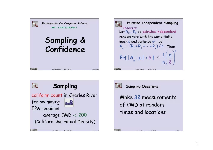
Pairwise Independent Sampling Let R1,…,Rn be pairwise independent random vars with the same finite mean μ and variance σ2. Let Then

A

n ::= (R1 + R2 +.+ R n) /

n.

Pr[ |An - µ |> δ ] ≤ 1 n σ δ      

2

Theorem:

Albert R Meyer, Ma y 13, 2013 confidence.3

coliform count in Charles River for swimming EPA requires average CMD < 200 (Coliform Microbial Density)

Sampling

Albert R Meyer, Ma y 13, 2013 confidence.4

Sampling Questions

Make 32 measurements

• f CMD at random

times and locations

1

Then

Albert R Meyer, Ma y 13, 2013 confidence.5

Sampling Questions

A few of the 32 counts turn out to be > 200 but their average is 180. Convince the EPA that avg in whole river is < 200?

Albert R Meyer, Ma y 13, 2013 confidence.6

Sampling Questions

That is, convince EPA that the estimate based on 32 samples is within 20 of the actual average?

Albert R Meyer, Ma y 13, 2013

Sampling parameters

confidence.7

c ::= actual average CMD in river

CMD sample ↔ ran var with μ = c n samples ↔ n mutually indep ran vars with μ = c

An ::= avg of the n CMD samples

Albert R Meyer, Ma y 13, 2013

Pr[|An - µ |> δ] ≤ 1 n σ δ      

2

Pairwise Independent Sampling

n = 32, µ = c, δ = 20

confidence.8

2

Albert R Meyer, May 13, 2013

Pr[A32 -c|> 20 ] ≤ 1 32 σ 20      

2

Pairwise Independent Sampling

n = 32, µ = c, δ = 20

confidence.9

?? don’t know (

Albert R Meyer, May 13, 2013

suppose L is max possible difference of samples Bound for (

confidence.10

= 50 worst σ = L 2

n = 32, µ = c, δ = 20

Pr[A32 -c|> 20 ] ≤ 1 32 σ 20      

2

Albert R Meyer, May 13, 2013

Pairwise Independent Sampling

confidence.11

1 32 25 20      

2

< 0.05

Pr[ |A32 -c| ≤ 20] > 0.95

Pr[A32 -c|> 20 ] ≤

Albert R Meyer, May 13, 2013 confidence.12

Confidence

tempting to say: “the probability that c = 180 ± 20 is at least 0.95”

• -technically wrong!

−not Probable Reality

3

Albert R Meyer, May 13, 2013 confidence.13

c is the actual average in the river.

c is unknown,

but not a random variable!

Confidence

Albert R Meyer, May 13, 2013 confidence.14

The possible outcomes of our sampling process is a random

• variable. We can say that the

“ probability that our sampling process will yield an average that is ± 20 of the true average at least 0.95”

Confidence

Albert R Meyer, May 13, 2013 confidence.15

Tell the EPA that with probability 0.95 our estimate method for avg CMD will be within 20 of the actual avg, c, in the river. Confidence

Albert R Meyer, May 13, 2013 confidence.17

For simplicity we say that

c = 180 ± 20 at the 95% confidence level

Confidence

4

Confidence Confidence Moral: when you are told that some fact holds at a high confidence level, remember that a random experiment lies behind this claim. Ask yourself “what experiment?”

Albert R Meyer, Ma y 13, 2013 confidence.18

Moral: Also ask “Why am I hearing about this particular experiment? How many

• thers were tried and not

reported?” See http://xkcd.com/882/

Albert R Meyer, Ma y 13, 2013 confidence.19

5

MIT OpenCourseWare http://ocw.mit.edu

6.042J / 18.062J Mathematics for Computer Science

Spring 2015 For information about citing these materials or our Terms of Use, visit: http://ocw.mit.edu/terms.