RMSA: Resonance Frequency x W e W L L e ~ where m and n are - - PowerPoint PPT Presentation

RMSA: Resonance Frequency

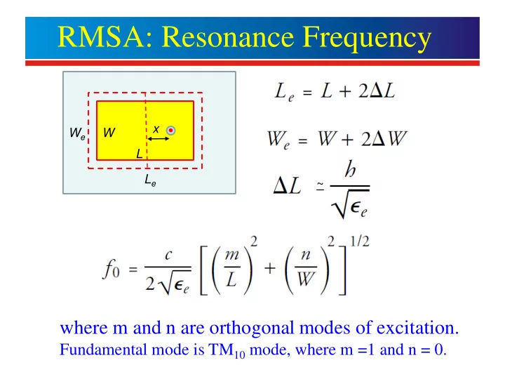
where m and n are orthogonal modes of excitation.

Fundamental mode is TM10 mode, where m =1 and n = 0.

L Le W We ~ x

RMSA – Characterization

RMSA: Design Equations

Smaller or larger W can be taken than the W obtained from this expression.

BW α W and Gain α W Choose feed-point x between L/6 to L/4.

RMSA: Design Example

Design a RMSA for Wi-Fi application (2.400 to 2.483 GHz)

Chose Substrate: εr = 2.32, h = 0.16 cm and tan δ = 0.001

= 3 x 1010 / ( 2 x 2.4415 x 109 x √1.66) = 4.77 cm. W = 4.7 cm is taken = 2.23 Le = 3 x 1010 / ( 2 x 2.4415 x 109 x √2.23) cm = 4.11 cm L = Le – 2 ∆L = 4.11 – 2 x 0.16 / √2.23 = 3.9 cm

RMSA: Design Example – Simulation using IE3D

L = 3.9 cm, W = 4.7 cm, x = 0.7 cm εr = 2.32, h = 0.16 cm and tan δ = 0.001 Zin = 54Ω at f = 2.414 GHz BW for |S11| < -10 dB is from 2.395 to 2.435 GHz = 40 MHz

Designed f = 2.4415 and Simulated f = 2.414 GHz % error = 1.1%. Also, BW is small.

SOLUTION: Increase h and reduce L

L = 3 cm and W = 4 cm

Substrate parameters: εr = 2.55, h = 0.159 cm, and tan δ = 0.001 Probe diameter = 0.12 cm for SMA connector. RMSA is analyzed using commercially available IE3D software.

Effect of Various Parameters on Performance of RMSA

L Le W We x

Effect of Feed Point Location (x)

For Infinite Ground Plane

With increase in x, input impedance plot shifts right towards higher impedance values.

Rectangular Microstrip Antenna (RMSA)

Co-axial feed Side View r Ground plane h Top View L W X Y x

Effect of Width (W)

With increase in W, aperture area, εe and fringing fields increase, hence frequency decreases and input impedance plot shifts towards lower impedance values.

BW α W and Gain α W

Effect of Thickness (h)

However, to reduce surface waves As h increases, fringing fields and probe inductance increase, frequency decreases and input impedance plot shifts upward.

BW α h/λ0

Effect of Probe Diameter

As probe diameter decreases, its inductance increases, so resonance frequency decreases and input impedance locus moves upward to the inductive region.

Effect of Loss Tangent (tanδ )

With increase in tan δ, dielectric losses increase, so input impedance locus moves left towards lower impedance

• value. BW increases but efficiency and gain decrease.

Effect of Dielectric Constant (εr)

With decrease in εr, both L and W increase, which increases fringing fields and aperture area, hence both BW and Gain increase.

RMSA – Pattern for Different εr (TM10 mode)

With increase in εr , size of the antenna decreases for same resonance frequency. Hence, gain decreases and HPBW increases.

RMSA – Pattern for Different εr (TM30 mode)

For TM30 mode, Le = 3 λ0 / (2 √ εe )

For εr = 2.32, Le ~ λ0 So, two radiating slots will be at a distance of λ0 yielding grating lobe in E-plane.

RMSA – Dual Polarization (TM10 and TM01 modes)

L = 10.1 cm and W = 7.9 cm Orthogonal Feeds at: x = 3.8 cm and y = 2.9 cm Substrate Parameters: εr = 4.3, h = 0.16 cm, tanδ = 0.02

( - - - ) theoretical, (——) measured

Measured resonance frequencies are 712 MHz and 913 MHz for two orthogonal modes

Effect of Finite Ground Plane

Finite Ground Plane Size is taken as Lg = L + 6h + 6h and Wg = W + 6h + 6h

MSA – BW Variation with h and f

Square MSA in Air – VSWR Plot

Square MSA on a finite ground plane. Low cost - Metallic plate suspended in air and fed by a co-axial feed. BW for VSWR < 2 is 95 MHz at 1.8 GHz (% BW ~ 5%)

Square MSA in Air – Radiation Pattern

Radiation Pattern at 1.8 GHz

F/B = 15 dB Cross Polar < 20 dB

MSA – Suspended Configurations

CMSA: Resonance Frequency

where Knm is the mth root

• f the derivative of the

Bessel function of order n For Fundamental TM11 Mode: f0 ~ 8.791 / [(a + h/ √εr) √εe ] GHz where a and h are in cm and εe < εr Design Equation: a ~ 8.791 / (f0 √εe) - h /√εr

Choose feed-point x between 0.3a to 0.5a