Risk Adjusted Inflation Indices James Jay R Black, CCEA Operations - - PowerPoint PPT Presentation

risk adjusted inflation indices
SMART_READER_LITE
LIVE PREVIEW

Risk Adjusted Inflation Indices James Jay R Black, CCEA Operations - - PowerPoint PPT Presentation

Risk Adjusted Inflation Indices James Jay R Black, CCEA Operations Research Analyst / Cost Team Leader Naval Sea Systems Command Cost Engineering and Industrial Analysis Division (NAVSEA 05C) Presented at the 2014 ICEAA Professional


slide-1
SLIDE 1

Risk Adjusted Inflation Indices

James “Jay” R Black, CCEA Operations Research Analyst / Cost Team Leader Naval Sea Systems Command Cost Engineering and Industrial Analysis Division (NAVSEA 05C) Presented at the 2014 ICEAA Professional Development and Training Workshop June, 2014

slide-2
SLIDE 2

Introduction

  • It is often observed that Office of the Secretary of Defense

(OSD) inflation rates are different than prime contractor specific inflation rates seen in:

– Forward Pricing Rate Agreements/Proposals (FPRAs/FPRPs) – Commodity group composite rates (e.g. Global Insight indices).

  • Yet, it is a standard practice in many cost estimating
  • rganizations to use OSD inflation rates for escalating future-

year costs in estimates without giving consideration to a range

  • f different possible inflation rates
  • This can result in cost estimates that underestimate the

effects of inflation

– Especially for programs that have many years of procurement and/or

  • perations & support (where the compounding effects of inflation are

significant)

  • This presentation proposes an approach to create risk

adjusted inflation indices based on defined risk distributions, thus giving consideration to a range of different inflation rate possibilities

slide-3
SLIDE 3
  • Before sharing the proposed approach, I’d like

to share a different approach I’ve seen previously...

slide-4
SLIDE 4

Discreet Distributions on Weighted Indices

  • One approach that has been used to model uncertainty
  • n future-year inflation is to define discreet

distributions on the weighted indices for each individual year, for example:

– FY20 Weighted Index = distribution(parameter1, parameter2,…) – FY19 Weighted Index = distribution(parameter1, parameter2,…) – FY18 Weighted Index = distribution(parameter1, parameter2,…) – FY17 Weighted Index = distribution(parameter1, parameter2,…) – FY16 Weighted Index = distribution(parameter1, parameter2,…) – Where the most likely value is usually the OSD weighted index for that year

  • This approach has limitations…
slide-5
SLIDE 5

Discreet Distributions on Weighted Indices (cont.)

  • This approach has limitations:

– The cumulative effect of the uncertainty around all the weighted indices cannot be easily compared to the other cost risk drivers

  • I.e., “If FY16-20 Inflation were combined, where would it rank on the Tornado Chart?”
  • Often results in a tornado chart that resembles:

– Also, using discreet distributions on the weighted indices does not influence the compounding effect of each year’s inflation rate on the following years

  • I.e., the results of the risk simulation for FY16 do not affect FY17, FY18, and so on

$3.7 $3.9 $4.1 $4.3 $4.5 Mean Time Between Failure SW Maintenance Productivity Labor Rates FY20 Weighted Index FY19 Weighted Index FY18 Weighted Index FY17 Weighted Index FY16 Weighted Index

Notional O&S Tornado Chart

$$ $ $ $$ $$$

slide-6
SLIDE 6
  • On to the proposed approach…
slide-7
SLIDE 7
  • Let’s review how weighted indices are built up
  • Example OSD inflation table:
  • Here, the weighted index for 2004 is generated using the ratio method
  • Also, note that OSD future-year inflation rate %’s are all the same

– I.e. from FY15 and onward, every year is 1.9%

YEAR1 YEAR2 YEAR3 YEAR4 YEAR5 YEAR6 Total 2004 2.00% 1.000 57.4% 32.7% 4.6% 2.4% 1.2% 1.7% 100.0% 1.017 2005 2.80% 1.028 58.6% 32.2% 4.3% 2.2% 1.1% 1.6% 100.0% 1.045 2006 3.10% 1.060 61.0% 29.8% 4.3% 2.2% 1.1% 1.6% 100.0% 1.074 2007 2.70% 1.088 57.5% 33.3% 4.3% 2.2% 1.1% 1.6% 100.0% 1.102 2008 2.40% 1.115 53.6% 37.9% 4.8% 2.1% 1.6% 0.0% 100.0% 1.124 2009 1.50% 1.131 48.6% 42.3% 5.1% 2.3% 1.7% 0.0% 100.0% 1.139 2010 0.80% 1.140 53.4% 38.3% 4.7% 2.1% 1.6% 0.0% 100.0% 1.154 2011 2.00% 1.163 31.4% 60.4% 4.6% 2.1% 1.5% 0.0% 100.0% 1.181 2012 1.80% 1.184 31.4% 60.4% 4.6% 2.1% 1.5% 0.0% 100.0% 1.204 2013 2.10% 1.209 31.4% 60.4% 4.6% 2.1% 1.5% 0.0% 100.0% 1.228 2014 1.90% 1.232 31.4% 60.4% 4.6% 2.1% 1.5% 0.0% 100.0% 1.251 2015 1.90% 1.255 31.4% 60.4% 4.6% 2.1% 1.5% 0.0% 100.0% 1.275 2016 1.90% 1.279 31.4% 60.4% 4.6% 2.1% 1.5% 0.0% 100.0% 1.299 2017 1.90% 1.304 31.4% 60.4% 4.6% 2.1% 1.5% 0.0% 100.0% 1.324 2018 1.90% 1.328 31.4% 60.4% 4.6% 2.1% 1.5% 0.0% 100.0% 1.349 2019 1.90% 1.354 31.4% 60.4% 4.6% 2.1% 1.5% 0.0% 100.0% 1.374 2020 1.90% 1.379 31.4% 60.4% 4.6% 2.1% 1.5% 0.0% 100.0% 1.401 Weighted Index Outlay Phasing Fiscal Year Inflation Rate % Raw Index

Building Weighted Indices 101

1

n

(Oi / Ii)

i=1

Weighted Index = I = Raw Index O = Outlay Phasing % n = number of years in outlay profile

slide-8
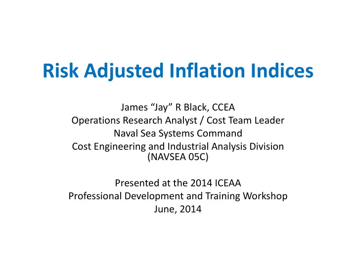
SLIDE 8

YEAR1 YEAR2 YEAR3 YEAR4 YEAR5 YEAR6 Total 2015 1.255 31.4% 60.4% 4.6% 2.1% 1.5% 0.0% 100% 1.275 2016 1.279 31.4% 60.4% 4.6% 2.1% 1.5% 0.0% 100% 1.299 2017 1.304 31.4% 60.4% 4.6% 2.1% 1.5% 0.0% 100% 1.324 2018 1.328 31.4% 60.4% 4.6% 2.1% 1.5% 0.0% 100% 1.349 2019 1.354 31.4% 60.4% 4.6% 2.1% 1.5% 0.0% 100% 1.374 2020 1.379 31.4% 60.4% 4.6% 2.1% 1.5% 0.0% 100% 1.401 Weighted Index Outlay Phasing Fiscal Year Raw Index Inflation Rate %

Each Year's Inflation % is set to the

  • utput of the

risk simulation

Proposed Approach

  • The proposed approach is for future-year escalation only

– Prior year escalation rates are actuals (i.e. can’t change the past)

  • The proposed approach is to:

– Define a single distribution for all the future-year inflation rates of that appropriation type – Then, assign the output of the risk simulation on that distribution to each year’s inflation rate % – For example:

  • Composite Inflation Risk = distribution(parameter1, parameter2,…)

These weighted indices are now risk adjusted

slide-9
SLIDE 9

Proposed Approach

  • This approach produces a tornado chart where the cumulative

effect of the uncertainty around all the weighted indices can be compared to the other cost risk drivers:

  • Also, modeling uncertainty with this approach influences the

compounding effect of each year’s rate on the following years

– I.e., the FY15 raw index, affects FY16, which affects FY17 and so on

$3.7 $3.9 $4.1 $4.3 $4.5 Composite Inflation Risk Mean Time Between Failure SW Maintenance Productivity Labor Rates

Notional O&S Tornado Chart

$$ $ $ $$ $$$

slide-10
SLIDE 10

Don’t Forget..

  • As with any cost risk analysis, make sure to

assign correlation between each distribution

slide-11
SLIDE 11

Acknowledgments

  • Thank you to the following individuals for

their inputs to this presentation:

– Jake Mender of the Naval Center for Cost Analysis – Tim Lawless and Lisa Pfeiffer of the Naval Sea Systems Command Cost Engineering and Industrial Analysis Division (NAVSEA 05C)