RICARDIAN MODEL Simplest and earliest (1817) complete model of - - PowerPoint PPT Presentation

ECO 352 – Spring 2010

• No. 5 – Feb. 16

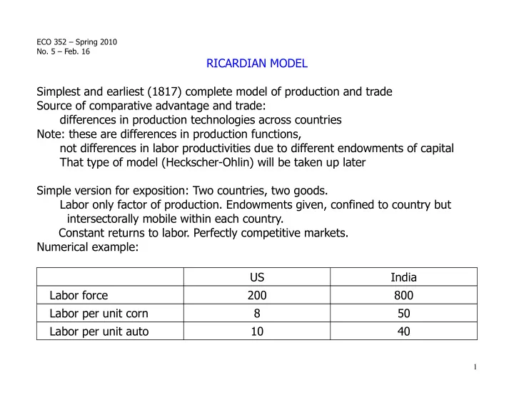
RICARDIAN MODEL Simplest and earliest (1817) complete model of production and trade Source of comparative advantage and trade: differences in production technologies across countries Note: these are differences in production functions, not differences in labor productivities due to different endowments of capital That type of model (Heckscher-Ohlin) will be taken up later Simple version for exposition: Two countries, two goods. Labor only factor of production. Endowments given, confined to country but intersectorally mobile within each country. Constant returns to labor. Perfectly competitive markets. Numerical example: US India Labor force 200 800 Labor per unit corn 8 50 Labor per unit auto 10 40

1

PRODUCTION POSSIBILITY FRONTIERS PPFs in the two countries: Supply in the two countries:

2

Corn Autos Autos U.S. India 20 25 20 16 slope = 0.8 slope = 1.25 Corn Corn Autos Autos U.S. India 20 25 20 16 slope < 0.8 slope > 1.25 Corn slope > 0.8 slope < 1.25

Notation: P = PC /PA , relative price of corn, R = QC /QA , relative quantity of corn Production and supply: US: If P < 0.8, QC = 0, QA = 20, R = QC /QA = 0. If P = 0. 8, QC , QA can be anywhere on PPF, 0 < QC /QA < ∞. If P > 0.8, QC = 25, QA = 0, R = QC /QA = ∞. India similar, with crucial value of P = 1.25. Autarkic equilibria in two countries: Relative price of corn is lower in the US, relative quantity consumed is higher.

3

US India P R R P 0.8 1.25 RS RS RD RD

TRADE Relative supply: When P < 0.8, both countries produce only autos, world ratio R = 0 When 0.8 < P < 1.25, US produces 25 corn, India produces 20 autos, R = 1.25 When P > 1.25, both countries produce only corn, R = ∞. When P = 0.8, India produces 20 autos. US varies between 20 autos, no corn (world R = 0), and 0 autos, 25 corn (world R = 1.25) When P = 1.25, similarly world R can be anywhere between 1.25 and ∞. Depending on position

• f relative demand, the

trading equilibrium can be

• ne of three types:

complete specialization (B)

• r incomplete (A, C).

A: P = 0.8. US produces both goods, India autos B: 0.8 < P < 1.25, US produces only corn, India only autos C: P = 1.25. US produces only corn, India produces both goods.

4

P R 0.8 1.25 RS RD RD RD A B C

A B C

EFFICIENT PRODUCTON AND WORLD PPF Suppose initially all labor produces autos in both (40 in all). If any corn is to be produced, it is better to do so by switching some labor in the US: each auto not produced releases 10 labor which can then produce 10/8 = 1.25 corn. In India each less auto yields only 40/50 = 0.8 more corn. Only when all US labor has been diverted to producing corn should any Indian labor be switched. Conversely, starting with all corn (41 units), to produce any autos, Indian labor should be switched. This despite the US producing autos more efficiently than India: only 10 units of labor against 40. The reason: the US produces corn even more efficiently: only 8 units of labor against 50. What matters is the ratio: 10/8 > 40/50, or 10/40 > 8/50. World PPF: juxtapose the country PPFs as the outer (thicker) lines. “Wrong” assignment of production would yield the less efficient inner (dashed) lines.

5

Autos Corn 40 20 25 41 World

If preferences are identical and homothetic everywhere, we can draw world indifference curves. Depending on their shape, three types of outcomes: A: US produces both goods India produces only autos B: US produces only corn India produces only autos C: US produces only corn India produces both goods Relative price of corn = slope of PPF 0.8 in A, 1.25 in C between 0.8 and 1.25 in B To sum up: Equilibrium/efficient pattern of production determined by comparative, not absolute advantage. Absolute advantage: Lower labor requirement per unit of output Comparative advantage: Country R has comparative advantage over country B in good X as against good Y if the ratio of unit labor requirement for X to that for Y is smaller in country R than in country B.

6

Autos Corn 40 20 25 41 World

A B C

WAGES Under constant returns to scale, P = MC = AC for each good produced, < if not produced. Autarky: US produces both goods: PU,A

C = 8 WU,A, PU,A A = 10 WU,A

Each US worker can buy WU,A/ PU,A

C = 1/8 corn, or WU,A/ PU,A A = 1/10 auto

India produces both goods: PI,A

C = 50 WI,A, PI,A A = 40 WI,A

Each Indian worker can buy WI,A/ PI,A

C = 1/50 corn, or WI,A/ PI,A A = 1/40 auto

Free trade: Consider type B equilibrium. For definiteness, let PT

C /PT A = 1 PT C = PT A

Important: No country label here; world market for goods, same price US produces only corn: PT

C = 8 WU,T, PT A < 10 WU,T

Each US worker can buy WU,T/ PT

C = 1/8 corn, or WU,T/ PT A > 1/10 auto

India produces only autos: PT

C < 50 WI,T, PT A = 40 WI,T

Each Indian worker can buy WI,T/ PT

C > 1/50 corn, or WI,T/ PT A = 1/40 auto

Labor in both countries is better off in trade than in autarky: can buy more of the good no longer produced. Benefit of trade: ability to buy cheaper imports! In A, C types, the country producing both goods has no gain, but no loss either.

7

Main findings: [1] Rival claims: US: We can't compete with low-wage Indian labor India: We can't compete with highly productive US labor are both wrong: Wages adjust; US continues to compete in corn, India in autos. [2] This model has only one factor in each country, and mobile across sectors: therefore no distributive conflict over trade. Reminder: different models have different uses. This one is useful for clarifying the idea of comparative advantage in the simplest way. [3] Absolute advantage does matter: it affects the standard of living. Here each US worker can buy much more than each Indian worker, whether we compare the two in autarky, or compare them with trade. But it does not matter for determining which goods to produce where, and therefore for the pattern of trade, nor for existence of gains from trade. Distinct comparisons: (a) Is US richer than India? Absolute advantage is relevant. (b) Does US gain from trade with India? Comparative advantage is relevant. [4] Different types A, B, C of equilibria also can arise for supply side reasons: (one country much larger or much more productive than the other).

8

GENERAL ALGEBRAIC RESTATEMENT Notation: Countries Home and Foreign; foreign variables denoted by asterisks. Trading prices etc. denoted by superscript T. Labor endowments L, L* . Wages W, W* Two goods X and Y. Prices PX , PY Unit labor inputs AX , AY in home, A*X , A*Y in Foreign. (Conversely, 1/AX etc. are labor productivity parameters.) Choose labels so that AX / AY < A*X / A*Y (equivalently AX / A*X < AY / A*Y ) This is the definition here of home having comparative advantage in X Relative price of X: P = PX/PY , Relative quantity ratio R = X/Y. Home PPF: AX X + AY Y = L, slope AX / AY Foreign PPF: A*X X* + A*Y Y* = L*, slope A*X/A*Y Relative demands identical, X/Y = f(PX/PY).

9

AUTARKY: Home: PX = W AX , PY = W AY ; W/PX = 1/AX , W/PY = 1/AY ; P = AX / AY Foreign: P*X = W* A*X, P*Y = W* A*Y; W*/P*X = 1/A*X, W*/P*Y = 1/A*Y ; P* = A*X/A*Y So Home has lower relative price of X in autarky than does Foreign: comparative advantage concept again. TRADE: Common price PT = PT

X / PT Y

(Note: each country may use different currencies / units of account so both prices in one may be equiproportionately higher than in the other.) Home produces X, may or may not produce Y. Foreign produces Y, may or may not produce X. Home: PT > AX / AY ; PT

X = WT AX , PT Y < WT AY ; WT/PT X = 1/AX , WT/PT Y > 1/AY

Foreign: PT < A*X / A*Y; PT

X < W*T A*X, PT Y = W*T A*Y; W*T/ PT X > 1 / A*X, W*T/ PT Y = 1 / A*Y

Exercise: Reconfirm the findings of the numerical example in this more general algebraic formulation.

10