Report ESRF and ILL summer school 2017 Introduction As a - PDF document

Synne Myhre ESRF and ILL summer school 2017 Report ESRF and ILL summer school 2017 Introduction As a conclusion of my participation to the ESRF and ILL summer school, this rapport will summarize the practical part of my stay. I participated in the work done at the ID02 at the ESRF. ID02 is a beamline for investigating soft matter. It combines wide angle x-ray scattering (WAXS) to ultra small angle x-ray scattering (USAXS) to explore all dimensions of soft matter systems. The non-equilibrium dynamics of soft matter and related systems can be explored down to a sub-millisecond range at this beamline. . Figure 1: Illustration of the regime of WAXS, SAXS and USAXS, as well as their microscopy alternatives. 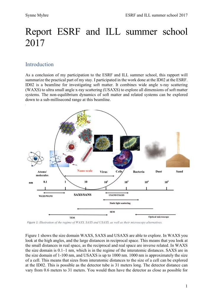Figure 1 shows the size domain WAXS, SAXS and USAXS are able to explore. In WAXS you look at the high angles, and the large distances in reciprocal space. This means that you look at the small distances in real space, as the reciprocal and real space are inverse related. In WAXS the size domain is 0.1–1 nm, which is in the regime of the interatomic distances. SAXS are in the size domain of 1-100 nm, and USAXS is up to 1000 nm. 1000 nm is approximately the size of a cell. This means that sizes from interatomic distances to the size of a cell can be explored at the ID02. This is possible as the detector tube is 31 meters long. The detector distance can vary from 0.6 meters to 31 meters. You would then have the detector as close as possible for 1

Synne Myhre ESRF and ILL summer school 2017 WAXS, and as far away as possible for USAXS. Figure 1 also shows the regime the competing microscopy methods are able to explore. The small angles in SAXS means that you look at angles below 6°. Advantages of WAXS/SAXS/USAXS over microscopy methods is that they can be done in situ in solution, and that you get an average over the whole sample, and not just information about parts of it. 2. Theory and methods Theoretical background The theory explained in this section is found here ( [1] [2] [3] [4]). Scattering Figure 1: Illustration of the scattering of a sample into a detector. In a scattering experiment the incident beam hits the sample with a given wavelength. SAXS is an elastic scattering technique, which means that no energy is lost in the scattering process. The incident wave of photons makes the electrons in the sample oscillate due to their electromagnetic field, and in this process the oscillating electrons will emit photons. In an elastic scattering process, the modulus of the wave vector of the incident and scattered beam is the same. $% 𝑙 " = Eq. 1 & ' $% 𝑙 ( = Eq. 2 & ) In Eq. 1 , and Eq. 2 , k is the wave vector and 𝜇 is the wavelength. As 𝑙 ( = 𝑙 " for an elastic process, this means that 𝜇 " = 𝜇 ( . The intensity measured at the detector as counts per seconds per pixel is given by 56 𝐽 - = 𝑗 / 𝑈 1 𝜁∆𝛻 57 Eq. 3 2

Synne Myhre ESRF and ILL summer school 2017 where 𝑗 / is the incident flux of X-ray photons, 𝑈 1 is the transmission, 𝜁 is the efficiency, ∆𝛻 is 56 the solid angle and 57 is the differential scattering cross section. The differential scattering cross section iIs the only variable that is not fixed in the equation, and therefore what we measure. The differential scattering cross section is the probability of a particle of the incident beam being scattered out from the unit sample into the solid angle. 59 : 56 𝐽 𝑟 = 57 = 57 Eq. 4 ; )<=> Eq. 4 is the differential scattering cross section normalized to volume sample ( 𝑊 (@AB ) , and is illustrated in Figure 2. Figure 2: Illustration of the differential scattering cross section. An incoming particle is scattered out from the scattering center into a solid angle. In the following a derivation from the wave vectors k s and k i into the well know relation D% H 𝑅 = & sin $ will be done. Q is the momentum transfer and is equal to 𝑅 = 𝑙 ( − 𝑙 " Eq. 5 so 𝑅 = 𝑙 ( − 𝑙 " Eq. 6 3

Synne Myhre ESRF and ILL summer school 2017 i in the figure, k s as k u f and 𝜄 as the Figure 3: The scattering of the incoming photon with demonstration of the vectors k i as k u angle between them. If we take the square of this we get 𝑅 $ = 𝑙 ( − 𝑙 " $ = 𝑙 ( $ − 2𝑙 ( 𝑙 " + 𝑙 " $ Eq. 7 The angle between the two wave vectors is given by 𝜄 , as shown in Figure 3. From simple geometry, we then have that 𝑅 $ = 𝑙 ( $ − 2 𝑙 ( 𝑙 " 𝑑𝑝𝑡 𝜄 + 𝑙 " $ Eq. 8 From the assumption that we have elastic scattering we have that 𝑙 ( = 𝑙 " so we can rewrite to $ − 2 𝑙 " 𝑅 $ = 2 𝑙 " $ 𝑑𝑝𝑡 𝜄 = 2 𝑙 " $ (1 − 𝑑𝑝𝑡 𝜄) Eq. 9 from Eq. 1 and Eq. 2 we have the formula for the wave vector which gives us $ $% S 𝑅 $ = (1 − 𝑑𝑝𝑡 𝜄) Eq. 10 & S From geometry, we have that 1 − cos 𝜄 = 2 sin $ H $ , so $ $% S 𝑅 $ = 2 𝑡𝑗𝑜 $ H $ Eq. 11 & S D% H 𝑅 = & ∗ 𝑡𝑗𝑜 $ Eq. 12 which is the expression for the scattering vector. This is inversely related to the distance by $% 𝑒 = Eq. 13 Y 4

Synne Myhre ESRF and ILL summer school 2017 The intensity we measure is given by 57 = 𝑜 ∗ ∆𝜍 ∗ 𝑊 $ ∗ 𝑄 𝑅 ∗ 𝑇(𝑅) : 56 𝐽 𝑅 = ; ∗ Eq. 14 : 56 ; ∗ where 57 is the differential scattering cross section normalized to volume, V. n is the particle number density, ∆𝜍 is the difference in contrast. For x rays, this is the difference in the electron density between the particles and the solvent. 𝑊 is the volume of the sample, 𝑄 𝑅 is the form factor of the particles, and 𝑇(𝑅) is the structure factor. The form factor tells about the size and shape of the scattering object, while the structure factor tells about the interactions between the particles in the sample. The density of the material is given by ] ' 𝜍 = ; ^=_>'<`a Eq. 15 where 𝑐 " is the scattering length and is given by Eq. 16 , and 𝑊 cA1B"@de is the molecular volume of the sample. e S 𝑐 " = D%f g - a @ S ∗ 𝑔 : Eq. 16 In Eq. 16 , e is the electron charge, 𝜁 / is the permittivity of free space, 𝑛 e is the electron mass, c is the speed of light and 𝑔 : is the is the real part of the atomic scattering factor. Each point of the particle gives rise to a scattered wave which can be expressed as 𝑓 "k1 , where q is expressed as a vector and r position vector of the point under consideration. In order to get the full scattering amplitude for the particle, one has to add up all the waves. The intensity is then the absolute square of the scattering amplitude. Because what we measure is the intensity, which is the amplitude squared, the phase information is lost. This means that there is not possible to go back the same way, by finding the amplitude, then do a Fourier transform to find the electron density, as shown in Figure 4. Therefore, one needs to make a model for the system, and fit it to the experimental data. 5

Synne Myhre ESRF and ILL summer school 2017 Figure 4: Illustration of the real space quantities electron density and autocorrelation function, and the inverse space quantities scattering amplitude and scattering intensity. The figure also shows in which direction Fourier transform is possible. Illustration taken from “Ilavsky_SAXS_Introduction_ACA-2.pdf”. Based on the shape and size of the particles in the sample, they will scatter the incoming x rays differently. This is what is meant by the form factor. Figure 5 shows the scattering pattern of a sphere. Based on how the intensity varies with Q, we can find what kind of shape and size the particles have in dilute solutions. We want to find the form factor in dilute solutions, as the distances between the particles then are so long so that they do not interact. The structure factor shown in Eq. 14 is then set to 1. Figure 5: Snapshot from a frame taken at ID02. When doing a scattering experiment, the results should be reduced to only contain scattering from the particles in the solution. Figure 6: Illustration of dividing up the scattering contributions from a sample into the scattering from the container, solvent and particles. 6