relational normalization theory
play

Relational Normalization Theory Chapter 6 1 Limitations of E-R - PDF document

Relational Normalization Theory Chapter 6 1 Limitations of E-R Designs Provides a set of guidelines, does not result in a unique database schema Does not provide a way of evaluating alternative schemas Normalization theory


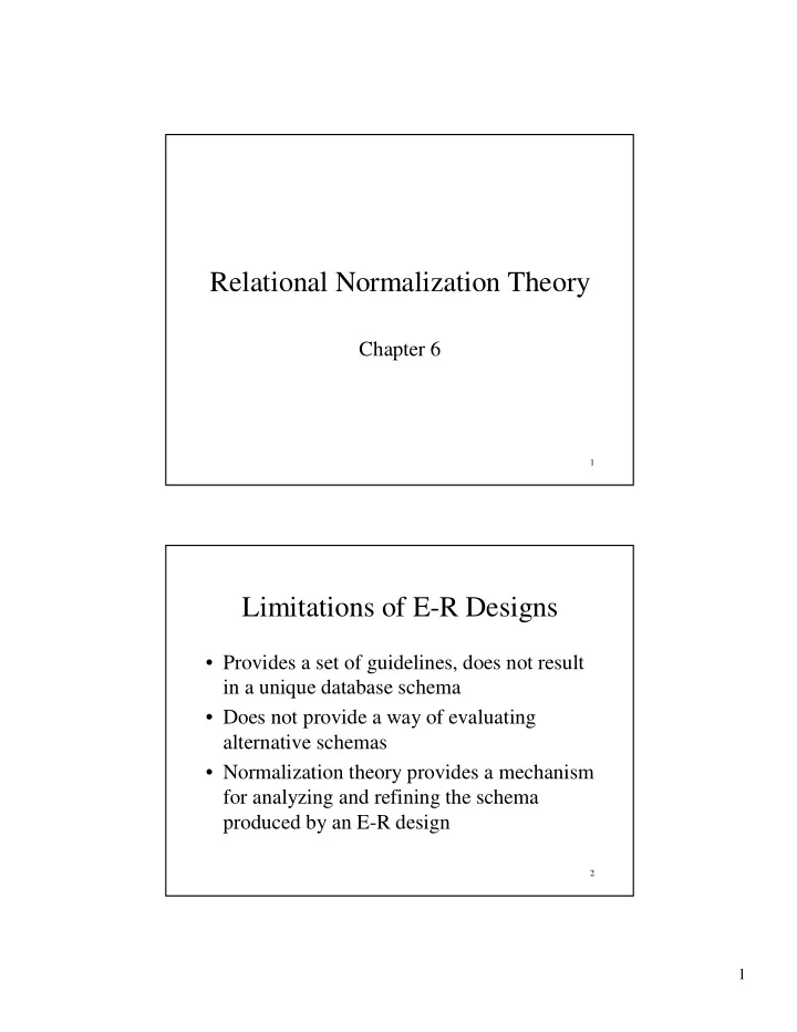
  1. Relational Normalization Theory Chapter 6 1 Limitations of E-R Designs • Provides a set of guidelines, does not result in a unique database schema • Does not provide a way of evaluating alternative schemas • Normalization theory provides a mechanism for analyzing and refining the schema produced by an E-R design 2 1
  2. Redundancy • Dependencies between attributes cause redundancy – Ex. All addresses in the same town have the same zip code SSN Name Town Zip Redundancy 1234 Joe Stony Brook 11790 4321 Mary Stony Brook 11790 5454 Tom Stony Brook 11790 …………………. 3 Redundancy and Other Problems • Set valued attributes in the E-R diagram result in multiple rows in corresponding table Person ( SSN, Name, Address, Hobbies ) • Example: Person – A person entity with multiple hobbies yields multiple rows in table Person Person • Hence, the association between Name and Address for the same person is stored redundantly – SSN is key of entity set, but ( SSN, Hobby ) is key of corresponding relation • The relation Person Person can’t describe people without hobbies 4 2

  3. Example ER Model SSN Name Address Hobby 1111 Joe 123 Main {biking, hiking} Relational Model SSN Name Address Hobby 1111 Joe 123 Main biking 1111 Joe 123 Main hiking ………… . Redundancy 5 Anomalies • Redundancy leads to anomalies: – Update anomaly : A change in Address must be made in several places – Deletion anomaly : Suppose a person gives up all hobbies. Do we: • Set Hobby attribute to null? No, since Hobby is part of key • Delete the entire row? No, since we lose other information in the row – Insertion anomaly : Hobby value must be supplied for any inserted row since Hobby is part of key 6 3

  4. Decomposition • Solution : use two relations to store Person Person information Person1 ( SSN, Name, Address ) – Person1 – Hobbies ( SSN, Hobby ) – Hobbies – • The decomposition is more general: people with hobbies can now be described • No update anomalies: – Name and address stored once – A hobby can be separately supplied or deleted 7 Normalization Theory • Result of E-R analysis need further refinement • Appropriate decomposition can solve problems • The underlying theory is referred to as normalization theory and is based on normalization theory functional dependencies (and other kinds, functional dependencies multivalued dependencies dependencies ) like multivalued 8 4

  5. Functional Dependencies • Definition: A functional dependency functional dependency (FD) on a relation schema R is a constraint X → Y , where X and Y are subsets of attributes of R. • Definition : An FD X → Y is satisfied satisfied in an instance r of R if for every pair of tuples, t and s: if t and s agree on all attributes in X then they must agree on all attributes in Y – Key constraint is a special kind of functional dependency: all attributes of relation occur on the right-hand side of the FD: • SSN → SSN, Name, Address 9 Functional Dependencies • Address → ZipCode – Stony Brook’s ZIP is 11733 • ArtistName → BirthYear – Picasso was born in 1881 • Autobrand → Manufacturer , Engine type – Pontiac is built by General Motors with gasoline engine • Author, Title → PublDate – Shakespeare’s Hamlet published in 1600 10 5

  6. Functional Dependency - Example • Consider a brokerage firm that allows multiple clients to share an account, but each account is managed from a single office and a client can have no more than one account in an office HasAccount ( AcctNum, ClientId, OfficeId ) – HasAccount – • keys are ( ClientId, OfficeId ), ( AcctNum, ClientId ) – Client, OfficeId → AcctNum – AcctNum → OfficeId • Thus, attribute values need not depend only on key values 11 Entailment, Closure, Equivalence • Definition : If F is a set of FDs on schema R and f is another FD on R , then F entails entails f if every instance r of R that satisfies every FD in F also satisfies f – Ex : F = {A → B, B → C} and f is A → C • If Town → Zip and Zip → AreaCode then Town → AreaCode • Definition : The closure closure of F , denoted F + , is the set of all FDs entailed by F • Definition : F and G are equivalent equivalent if F entails G and G entails F 12 6

  7. Entailment (cont’ d) • Satisfaction, entailment, and equivalence are semantic concepts – defined in terms of the actual relations in the “real world.” – They define what these notions are , not how to compute them • How to check if F entails f or if F and G are equivalent? – Apply the respective definitions for all possible relations? • Bad idea : might be infinite number for infinite domains • Even for finite domains, we have to look at relations of all arities – Solution : find algorithmic, syntactic ways to compute these notions • Important : The syntactic solution must be “correct” with respect to the semantic definitions • Correctness has two aspects: soundness soundness and completeness completeness – see later 13 Armstrong’s Axioms for FDs • This is the syntactic way of computing/testing the various properties of FDs • Reflexivity : If Y ⊆ X then X → Y (trivial FD) – Name, Address → Name • Augmentation : If X → Y then X Z → YZ – If Town → Zip then Town, Name → Zip, Name • Transitivity : If X → Y and Y → Z then X → Z 14 7

  8. Soundness sound : If an FD f: X → Y can be derived • Axioms are sound from a set of FDs F using the axioms, then f holds in every relation that satisfies every FD in F . • Example: Given X → Y and X → Z then X → XY Augmentation by X YX → YZ Augmentation by Y X → YZ Transitivity – Thus, X → Y Z is satisfied in every relation where both X → Y and X → Z are satisfied • Therefore, we have derived the union rule union rule for FDs: we can take the union of the RHSs of FDs that have the same LHS 15 Completeness complete: If F entails f , then f • Axioms are complete can be derived from F using the axioms • A consequence of completeness is the following (naïve) algorithm to determining if F entails f : – Algorithm Algorithm: Use the axioms in all possible ways – to generate F + (the set of possible FD’s is finite so this can be done) and see if f is in F + 16 8

  9. Correctness • The notions of soundness and completeness link the syntax (Armstrong’ s axioms) with semantics (the definitions in terms of relational instances) • This is a precise way of saying that the algorithm for entailment based on the axioms is “ correct” with respect to the definitions 17 Generating F + F AB → C union AB → BCD decomp aug A → D AB → BD AB → BCDE AB → CDE trans aug D → E BCD → BCDE Thus, AB → BD, AB → BCD, AB → BCDE, and AB → CDE are all elements of F + 18 9

  10. Attribute Closure • Calculating attribute closure leads to a more efficient way of checking entailment attribute closure of a set of attributes, X, • The attribute closure with respect to a set of functional dependencies, F , (denoted X + F ) is the set of all attributes, A , such that X → A F 2 if F 1 ≠ F 2 – X + F 1 is not necessarily the same as X + • Attribute closure and entailment : Algorithm: Given a set of FDs, F , then X → Y if and – Algorithm – F ⊇ Y only if X + 19 Example - Computing Attribute Closure X X F + F : AB → C A {A, D, E} A → D AB {A, B, C, D, E} D → E (Hence AB is a key) AC → B B {B} D {D, E} Is AB → E entailed by F ? Yes Is D → C entailed by F ? No Result : X F + allows us to determine FDs of the form X → Y entailed by F 20 10

  11. Computation of Attribute Closure X + F closure := X; // since X ⊆ X + F repeat old := closure; if there is an FD Z → V in F such that Z ⊆ closure and V ⊆ closure then closure := closure ∪ V until old = closure – If T ⊆ closure then X → T is entailed by F 21 Example: Computation of Attribute Closure Problem : Compute the attribute closure of AB with respect to the set of FDs : AB → C (a) A → D (b) D → E (c) AC → B (d) Solution : Initially closure = {AB} Using (a) closure = {ABC} Using (b) closure = {ABCD} Using (c) closure = {ABCDE} 22 11

  12. Normal Forms • Each normal form is a set of conditions on a schema that guarantees certain properties (relating to redundancy and update anomalies) • First normal form (1NF) is the same as the definition of relational model (relations = sets of tuples; each tuple = sequence of atomic values) • Second normal form (2NF) – a research lab accident; has no practical or theoretical value – won’t discuss third • The two commonly used normal forms are third normal form (3NF) and Boyce Boyce- -Codd Codd normal form normal form normal form (BCNF) 23 BCNF • Definition : A relation schema R is in BCNF if for every FD X → Y associated with R either – Y ⊆ X (i.e., the FD is trivial) or – X is a superkey of R • Example : Person1 Person1( SSN, Name, Address ) – The only FD is SSN → Name, Address – Since SSN is a key, Person1 Person1 is in BCNF 24 12

Download Presentation
Download Policy: The content available on the website is offered to you 'AS IS' for your personal information and use only. It cannot be commercialized, licensed, or distributed on other websites without prior consent from the author. To download a presentation, simply click this link. If you encounter any difficulties during the download process, it's possible that the publisher has removed the file from their server.

Recommend


More recommend