Regression Noise model and likelihood Given a dataset D = { x n , y - - PowerPoint PPT Presentation

Linear Regression

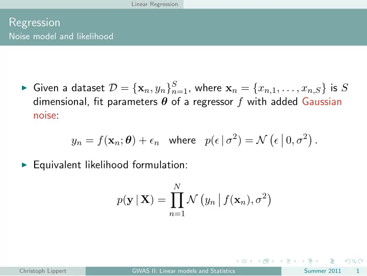
Regression

Noise model and likelihood

◮ Given a dataset D = {xn, yn}S n=1, where xn = {xn,1, . . . , xn,S} is S

dimensional, fit parameters θ of a regressor f with added Gaussian noise: yn = f(xn; θ) + ǫn where p(ǫ | σ2) = N

• ǫ
• 0, σ2

.

◮ Equivalent likelihood formulation:

p(y | X) =

N

• n=1

N

• yn
• f(xn), σ2

Christoph Lippert GWAS II: Linear models and Statistics Summer 2011 1

Linear Regression

Regression

Choosing a regressor

◮ Choose f to be linear:

p(y | X) =

N

• n=1

N

• yn
• xn · θ + c, σ2

◮ Consider bias free case, c = 0,

• therwise include an additional

column of ones in each xn.

Christoph Lippert GWAS II: Linear models and Statistics Summer 2011 2

Linear Regression

Regression

Choosing a regressor

◮ Choose f to be linear:

p(y | X) =

N

• n=1

N

• yn
• xn · θ + c, σ2

◮ Consider bias free case, c = 0,

• therwise include an additional

column of ones in each xn.

Equivalent graphical model Christoph Lippert GWAS II: Linear models and Statistics Summer 2011 2

Linear Regression

Linear Regression

Maximum likelihood

◮ Taking the logarithm, we obtain

ln p(y | θσ2) =

N

• n=1

ln N

• yn
• xn · θ, σ2

= −N 2 ln 2πσ2 − 1 2σ2

N

• n=1

(yn − xn · θ)2

• Sum of squares

◮ The likelihood is maximized when the squared error is minimized. ◮ Least squares and maximum likelihood are equivalent.

Christoph Lippert GWAS II: Linear models and Statistics Summer 2011 3

Linear Regression

Linear Regression

Maximum likelihood

◮ Taking the logarithm, we obtain

ln p(y | θσ2) =

N

• n=1

ln N

• yn
• xn · θ, σ2

= −N 2 ln 2πσ2 − 1 2σ2

N

• n=1

(yn − xn · θ)2

• Sum of squares

◮ The likelihood is maximized when the squared error is minimized. ◮ Least squares and maximum likelihood are equivalent.

Christoph Lippert GWAS II: Linear models and Statistics Summer 2011 3

Linear Regression

Linear Regression

Maximum likelihood

◮ Taking the logarithm, we obtain

ln p(y | θσ2) =

N

• n=1

ln N

• yn
• xn · θ, σ2

= −N 2 ln 2πσ2 − 1 2σ2

N

• n=1

(yn − xn · θ)2

• Sum of squares

◮ The likelihood is maximized when the squared error is minimized. ◮ Least squares and maximum likelihood are equivalent.

Christoph Lippert GWAS II: Linear models and Statistics Summer 2011 3

Linear Regression

Linear Regression and Least Squares

y x f(xn, w) y

n

xn

(C.M. Bishop, Pattern Recognition and Machine Learning)

E(θ) = 1 2

N

• n=1

(yn − xn · θ)2

Christoph Lippert GWAS II: Linear models and Statistics Summer 2011 4

Linear Regression

Linear Regression and Least Squares

◮ Derivative w.r.t a single weight entry θi

d dθi ln p(y | θ, σ2) = d dθi

• − 1

2σ2

N

• n=1

(yn − xn · θ)2

• ◮ Set gradient w.r.t. θ to zero

Christoph Lippert GWAS II: Linear models and Statistics Summer 2011 5

Linear Regression

Linear Regression and Least Squares

◮ Derivative w.r.t a single weight entry θi

d dθi ln p(y | θ, σ2) = d dθi

• − 1

2σ2

N

• n=1

(yn − xn · θ)2

• ◮ Set gradient w.r.t. θ to zero

Christoph Lippert GWAS II: Linear models and Statistics Summer 2011 5

Linear Regression

Linear Regression and Least Squares

◮ Derivative w.r.t a single weight entry θi

d dθi ln p(y | θ, σ2) = d dθi

• − 1

2σ2

N

• n=1

(yn − xn · θ)2

• ◮ Set gradient w.r.t. θ to zero

∇θ ln p(y | θ, σ2) = 1 σ2

N

• n=1

(yn − xn · θ)xT

n = 0

= ⇒ θML =?

Christoph Lippert GWAS II: Linear models and Statistics Summer 2011 5

Linear Regression

Linear Regression and Least Squares

◮ Derivative w.r.t. a single weight entry θi

d dθi ln p(y | θ, σ2) = d dθi

• − 1

2σ2

N

• n=1

(yn − xn · θ)2

• = 1

σ2

N

• n=1

(yn − xn · θ)xi

◮ Set gradient w.r.t. θ to zero

∇θ ln p(y | θ, σ2) = 1 σ2

N

• n=1

(yn − xn · θ)xT

n = 0

= ⇒ θML = (XTX)−1XT

• Pseudo inverse

y

◮ Here, the matrix X is defined as X =

  x1,1 . . . x1, S . . . . . . . . . xN,1 . . . xN,S  

Christoph Lippert GWAS II: Linear models and Statistics Summer 2011 6

Linear Regression

Linear Regression and Least Squares

◮ Derivative w.r.t. a single weight entry θi

d dθi ln p(y | θ, σ2) = d dθi

• − 1

2σ2

N

• n=1

(yn − xn · θ)2

• = 1

σ2

N

• n=1

(yn − xn · θ)xi

◮ Set gradient w.r.t. θ to zero

∇θ ln p(y | θ, σ2) = 1 σ2

N

• n=1

(yn − xn · θ)xT

n = 0

= ⇒ θML = (XTX)−1XT

• Pseudo inverse

y

◮ Here, the matrix X is defined as X =

  x1,1 . . . x1, S . . . . . . . . . xN,1 . . . xN,S  

Christoph Lippert GWAS II: Linear models and Statistics Summer 2011 6

Linear Regression

Linear Regression and Least Squares

◮ Derivative w.r.t. a single weight entry θi

d dθi ln p(y | θ, σ2) = d dθi

• − 1

2σ2

N

• n=1

(yn − xn · θ)2

• = 1

σ2

N

• n=1

(yn − xn · θ)xi

◮ Set gradient w.r.t. θ to zero

∇θ ln p(y | θ, σ2) = 1 σ2

N

• n=1

(yn − xn · θ)xT

n = 0

= ⇒ θML = (XTX)−1XT

• Pseudo inverse

y

◮ Here, the matrix X is defined as X =

  x1,1 . . . x1, S . . . . . . . . . xN,1 . . . xN,S  

Christoph Lippert GWAS II: Linear models and Statistics Summer 2011 6

Hypothesis Testing

Hypothesis Testing

Example:

◮ Given a sample

D = {x1, . . . , xN}.

◮ Test whether H0 : θs = 0 (null

hypothesis) or H1 : θs = 0 (alternative hypothesis) is true.

◮ To show that θs = 0 we can

perform a statistical test that tries to reject H0.

◮ type 1 error: H0 is rejected but

does hold.

◮ type 2 error: H0 is accepted

but does not hold.

Christoph Lippert GWAS II: Linear models and Statistics Summer 2011 7

Hypothesis Testing

Hypothesis Testing

Example:

◮ Given a sample

D = {x1, . . . , xN}.

◮ Test whether H0 : θs = 0 (null

hypothesis) or H1 : θs = 0 (alternative hypothesis) is true.

◮ To show that θs = 0 we can

perform a statistical test that tries to reject H0.

◮ type 1 error: H0 is rejected but

does hold.

◮ type 2 error: H0 is accepted

but does not hold.

Christoph Lippert GWAS II: Linear models and Statistics Summer 2011 7

Hypothesis Testing

Hypothesis Testing

Example:

◮ Given a sample

D = {x1, . . . , xN}.

◮ Test whether H0 : θs = 0 (null

hypothesis) or H1 : θs = 0 (alternative hypothesis) is true.

◮ To show that θs = 0 we can

perform a statistical test that tries to reject H0.

◮ type 1 error: H0 is rejected but

does hold.

◮ type 2 error: H0 is accepted

but does not hold.

Christoph Lippert GWAS II: Linear models and Statistics Summer 2011 7

Hypothesis Testing

Hypothesis Testing

Example:

◮ Given a sample

D = {x1, . . . , xN}.

◮ Test whether H0 : θs = 0 (null

hypothesis) or H1 : θs = 0 (alternative hypothesis) is true.

◮ To show that θs = 0 we can

perform a statistical test that tries to reject H0.

◮ type 1 error: H0 is rejected but

does hold.

◮ type 2 error: H0 is accepted

but does not hold.

H0 holds H0 doesn’t hold H0 accepted true negatives false negatives type-2 error H0 rejected false positives true positives type-1 error Christoph Lippert GWAS II: Linear models and Statistics Summer 2011 7

Hypothesis Testing

Hypothesis Testing

Example:

◮ Given a sample

D = {x1, . . . , xN}.

◮ Test whether H0 : θs = 0 (null

hypothesis) or H1 : θs = 0 (alternative hypothesis) is true.

◮ To show that θs = 0 we can

perform a statistical test that tries to reject H0.

◮ type 1 error: H0 is rejected but

does hold.

◮ type 2 error: H0 is accepted

but does not hold.

H0 holds H0 doesn’t hold H0 accepted true negatives false negatives type-2 error H0 rejected false positives true positives type-1 error Christoph Lippert GWAS II: Linear models and Statistics Summer 2011 7

Hypothesis Testing

Hypothesis Testing

◮ Given a sample

D = {x1, . . . , xN}.

◮ Test whether H0 : θs = 0 (null

hypothesis) or H1 : θs = 0 (alternative hypothesis) is true.

◮ The significance level α defines

the threshold and the sensitivity

• f the test. This equals the

probability of a type-1 error.

◮ Usually decision is based on a

test statistic.

◮ The critical region defines the

values of the test statistic that lead to a rejection of the test.

Christoph Lippert GWAS II: Linear models and Statistics Summer 2011 8

Hypothesis Testing

Hypothesis Testing

◮ Given a sample

D = {x1, . . . , xN}.

◮ Test whether H0 : θs = 0 (null

hypothesis) or H1 : θs = 0 (alternative hypothesis) is true.

◮ The significance level α defines

the threshold and the sensitivity

• f the test. This equals the

probability of a type-1 error.

◮ Usually decision is based on a

test statistic.

◮ The critical region defines the

values of the test statistic that lead to a rejection of the test.

Christoph Lippert GWAS II: Linear models and Statistics Summer 2011 8

Hypothesis Testing

Hypothesis Testing

◮ Given a sample

D = {x1, . . . , xN}.

◮ Test whether H0 : θs = 0 (null

hypothesis) or H1 : θs = 0 (alternative hypothesis) is true.

◮ The significance level α defines

the threshold and the sensitivity

• f the test. This equals the

probability of a type-1 error.

◮ Usually decision is based on a

test statistic.

◮ The critical region defines the

values of the test statistic that lead to a rejection of the test.

Christoph Lippert GWAS II: Linear models and Statistics Summer 2011 8

Hypothesis Testing

Hypothesis Testing

◮ Given a sample

D = {x1, . . . , xN}.

◮ Test whether H0 : θs = 0 (null

hypothesis) or H1 : θs = 0 (alternative hypothesis) is true.

◮ The significance level α defines

the threshold and the sensitivity

• f the test. This equals the

probability of a type-1 error.

◮ Usually decision is based on a

test statistic.

◮ The critical region defines the

values of the test statistic that lead to a rejection of the test.

Christoph Lippert GWAS II: Linear models and Statistics Summer 2011 8

Hypothesis Testing

Testing in Linear Regression

Likelihood Ratio Test

p(y | X) =

N

• n=1

N

• yn
• xn · θ + xn,sβ, σ2

◮ xn,s: SNP to be tested ◮ xn: regression covariates (including

bias term)

◮ Race ◮ Known background SNPs ◮ Environment Equivalent graphical model

xn: regression covariates

Christoph Lippert GWAS II: Linear models and Statistics Summer 2011 9

Hypothesis Testing

Testing in Linear Regression

Likelihood Ratio Test

p(y | X) =

N

• n=1

N

• yn
• xn · θ + xn,sβ, σ2

◮ xn,s: SNP to be tested ◮ xn: regression covariates (including

bias term)

◮ Race ◮ Known background SNPs ◮ Environment Equivalent graphical model

xn: regression covariates

Christoph Lippert GWAS II: Linear models and Statistics Summer 2011 9

Hypothesis Testing

Testing in Linear Regression

Likelihood Ratio Test

p(y | X) =

N

• n=1

N

• yn
• xn · θ + xn,sβ, σ2

◮ xn,s: SNP to be tested ◮ xn: regression covariates (including

bias term)

◮ Race ◮ Known background SNPs ◮ Environment Equivalent graphical model

xn: regression covariates

Christoph Lippert GWAS II: Linear models and Statistics Summer 2011 9

Hypothesis Testing

Testing in Linear Regression

Likelihood Ratio Test

p(y | X) =

N

• n=1

N

• yn
• xn · θ + xn,sβ, σ2

◮ Test H0 : β = 0 ◮ The ratio of the ML estimator and

the ML0 estimator restricted to H0 is a common test statistic.

Equivalent graphical model

xn: regression covariates

Christoph Lippert GWAS II: Linear models and Statistics Summer 2011 10

Hypothesis Testing

Testing in Linear Regression

Likelihood Ratio Test

p(y | X) =

N

• n=1

N

• yn
• xn · θ + xn,sβ, σ2

◮ Test H0 : β = 0 ◮ The ratio of the ML estimator and

the ML0 estimator restricted to H0 is a common test statistic.

Equivalent graphical model

xn: regression covariates

Christoph Lippert GWAS II: Linear models and Statistics Summer 2011 10

Hypothesis Testing

Testing in Linear Regression

Likelihood Ratio Test

p(y | X) =

N

• n=1

N

• yn
• xn · θ + xn,sβ, σ2

◮ Test H0 : β = 0 ◮ The ratio of the ML estimator and

the ML0 estimator restricted to H0 is a common test statistic. N

n=1 N

• yn
• xn · θML + xn,sβML, σ2

ML

• N

n=1 N

• yn
• xn · θML0 + xn,s0, σ2

ML0

• Equivalent graphical model

xn: regression covariates

Christoph Lippert GWAS II: Linear models and Statistics Summer 2011 10

Hypothesis Testing

P-value

definition

◮ Probability of observing a test statistic at least as extreme (e.g.

likelihood ratio statistic), given that H0 is true.

◮ Significance level α becomes threshold on P-value. ◮ Need to know the null distribution of test statistics. (usually

unknown)

◮ Possible to generate artificial null-distribution by permutations

Christoph Lippert GWAS II: Linear models and Statistics Summer 2011 11

Hypothesis Testing

P-value

definition

◮ Probability of observing a test statistic at least as extreme (e.g.

likelihood ratio statistic), given that H0 is true.

◮ Significance level α becomes threshold on P-value. ◮ Need to know the null distribution of test statistics. (usually

unknown)

◮ Possible to generate artificial null-distribution by permutations

Christoph Lippert GWAS II: Linear models and Statistics Summer 2011 11

Hypothesis Testing

P-value

definition

◮ Probability of observing a test statistic at least as extreme (e.g.

likelihood ratio statistic), given that H0 is true.

◮ Significance level α becomes threshold on P-value. ◮ Need to know the null distribution of test statistics. (usually

unknown)

◮ Possible to generate artificial null-distribution by permutations

Christoph Lippert GWAS II: Linear models and Statistics Summer 2011 11

Hypothesis Testing

P-value

definition

◮ Probability of observing a test statistic at least as extreme (e.g.

likelihood ratio statistic), given that H0 is true.

◮ Significance level α becomes threshold on P-value. ◮ Need to know the null distribution of test statistics. (usually

unknown)

◮ Possible to generate artificial null-distribution by permutations

Christoph Lippert GWAS II: Linear models and Statistics Summer 2011 11

Hypothesis Testing

P-value

Permutation procedure

Repeat M times:

◮ Permute phenotype y and

covariates x jointly over individuals.

◮ Compute permuted test statistic ◮ Add test statistic to emprirical null

distribution

Christoph Lippert GWAS II: Linear models and Statistics Summer 2011 12

Hypothesis Testing

P-value

Permutation procedure

Repeat M times:

◮ Permute phenotype y and

covariates x jointly over individuals.

◮ Compute permuted test statistic ◮ Add test statistic to emprirical null

distribution

covariates

Christoph Lippert GWAS II: Linear models and Statistics Summer 2011 12

Hypothesis Testing

P-value

Permutation procedure

Repeat M times:

◮ Permute phenotype y and

covariates x jointly over individuals.

◮ Compute permuted test statistic ◮ Add test statistic to emprirical null

distribution

covariates

Christoph Lippert GWAS II: Linear models and Statistics Summer 2011 12

Hypothesis Testing

P-value

Permutation procedure

Repeat M times:

◮ Permute phenotype y and

covariates x jointly over individuals.

◮ Compute permuted test statistic ◮ Add test statistic to emprirical null

distribution

covariates

Christoph Lippert GWAS II: Linear models and Statistics Summer 2011 12

Hypothesis Testing

P-value

Permutation procedure

Repeat M times:

◮ Permute phenotype y and

covariates x jointly over individuals.

◮ Compute permuted test statistic ◮ Add test statistic to emprirical null

distribution The P-value is the quantile of real test statistic in artificial null distribution.

covariates

Christoph Lippert GWAS II: Linear models and Statistics Summer 2011 12

Hypothesis Testing

Testing in Linear Regression

Likelihood Ratio Test revisited

◮ Can equivalently compute

log-likelihood ratio:

◮ Wilks’ theorem: 2LR follows a

Chi-square distribution with 1 degree of freedom.

◮ P-value = 1-CDF(2LR).

Equivalent graphical model

xn: regression covariates

Christoph Lippert GWAS II: Linear models and Statistics Summer 2011 13

Hypothesis Testing

Testing in Linear Regression

Likelihood Ratio Test revisited

◮ Can equivalently compute

log-likelihood ratio:

LR =

N

• n=1

log N

• yn
• xn · θML + xn,sβML, σ2

ML

• −

N

• n=1

log N

• yn
• xn · θML0, σ2

ML0

• ◮ Wilks’ theorem: 2LR follows a

Chi-square distribution with 1 degree of freedom.

◮ P-value = 1-CDF(2LR).

Equivalent graphical model

xn: regression covariates

Christoph Lippert GWAS II: Linear models and Statistics Summer 2011 13

Hypothesis Testing

Testing in Linear Regression

Likelihood Ratio Test revisited

◮ Can equivalently compute

log-likelihood ratio:

LR =

N

• n=1

log N

• yn
• xn · θML + xn,sβML, σ2

ML

• −

N

• n=1

log N

• yn
• xn · θML0, σ2

ML0

• ◮ Wilks’ theorem: 2LR follows a

Chi-square distribution with 1 degree of freedom.

◮ P-value = 1-CDF(2LR).

Christoph Lippert GWAS II: Linear models and Statistics Summer 2011 13

Hypothesis Testing

Testing in Linear Regression

Likelihood Ratio Test revisited

◮ Can equivalently compute

log-likelihood ratio:

LR =

N

• n=1

log N

• yn
• xn · θML + xn,sβML, σ2

ML

• −

N

• n=1

log N

• yn
• xn · θML0, σ2

ML0

• ◮ Wilks’ theorem: 2LR follows a

Chi-square distribution with 1 degree of freedom.

◮ P-value = 1-CDF(2LR).

Christoph Lippert GWAS II: Linear models and Statistics Summer 2011 13

Multiple Hypothesis Testing

Multiple Hypothesis Testing

Motivation

◮ Significance level α equals

probability of type-1 error.

◮ In GWAS we perform S = 106 tests ◮ At α = 0.01 we would expect 10000

type-1 errors!

◮ Probability of at least 1 type-1 error

is 1 − (1 − α)S → 1.

◮ Individual P-values < 0.01 are not

significant anymore.

H0 holds H0 doesn’t hold H0 accepted true negatives false negatives type-2 error H0 rejected false positives true positives type-1 error Christoph Lippert GWAS II: Linear models and Statistics Summer 2011 14

Multiple Hypothesis Testing

Multiple Hypothesis Testing

Motivation

◮ Significance level α equals

probability of type-1 error.

◮ In GWAS we perform S = 106 tests ◮ At α = 0.01 we would expect 10000

type-1 errors!

◮ Probability of at least 1 type-1 error

is 1 − (1 − α)S → 1.

◮ Individual P-values < 0.01 are not

significant anymore.

H0 holds H0 doesn’t hold H0 accepted true negatives false negatives type-2 error H0 rejected false positives true positives type-1 error Christoph Lippert GWAS II: Linear models and Statistics Summer 2011 14

Multiple Hypothesis Testing

Multiple Hypothesis Testing

Motivation

◮ Significance level α equals

probability of type-1 error.

◮ In GWAS we perform S = 106 tests ◮ At α = 0.01 we would expect 10000

type-1 errors!

◮ Probability of at least 1 type-1 error

is 1 − (1 − α)S → 1.

◮ Individual P-values < 0.01 are not

significant anymore.

H0 holds H0 doesn’t hold H0 accepted true negatives false negatives type-2 error H0 rejected false positives true positives type-1 error Christoph Lippert GWAS II: Linear models and Statistics Summer 2011 14

Multiple Hypothesis Testing

Multiple Hypothesis Testing

Motivation

◮ Significance level α equals

probability of type-1 error.

◮ In GWAS we perform S = 106 tests ◮ At α = 0.01 we would expect 10000

type-1 errors!

◮ Probability of at least 1 type-1 error

is 1 − (1 − α)S → 1.

◮ Individual P-values < 0.01 are not

significant anymore.

H0 holds H0 doesn’t hold H0 accepted true negatives false negatives type-2 error H0 rejected false positives true positives type-1 error Christoph Lippert GWAS II: Linear models and Statistics Summer 2011 14

Multiple Hypothesis Testing

Multiple Hypothesis Testing

Motivation

◮ Significance level α equals

probability of type-1 error.

◮ In GWAS we perform S = 106 tests ◮ At α = 0.01 we would expect 10000

type-1 errors!

◮ Probability of at least 1 type-1 error

is 1 − (1 − α)S → 1.

◮ Individual P-values < 0.01 are not

significant anymore.

H0 holds H0 doesn’t hold H0 accepted true negatives false negatives type-2 error H0 rejected false positives true positives type-1 error Christoph Lippert GWAS II: Linear models and Statistics Summer 2011 14

Multiple Hypothesis Testing

Multiple Hypothesis Testing

Motivation

◮ Significance level α equals

probability of type-1 error.

◮ In GWAS we perform S = 106 tests ◮ At α = 0.01 we would expect 10000

type-1 errors!

◮ Probability of at least 1 type-1 error

is 1 − (1 − α)S → 1.

◮ Individual P-values < 0.01 are not

significant anymore. Need to correct for multiple hypothesis testing!

H0 holds H0 doesn’t hold H0 accepted true negatives false negatives type-2 error H0 rejected false positives true positives type-1 error Christoph Lippert GWAS II: Linear models and Statistics Summer 2011 14

Multiple Hypothesis Testing

Multiple Hypothesis Testing

Family-Wise Error Rate (FWER)

◮ Probability of at least one type-2

error.

◮ Correct by bounding the FWER. ◮ Bonferroni correction: PB = P ∗ S ◮ Equivalently P < α

S significant.

◮ Bounds the FWER 1 − (1 − α/S)S

by α

H0 holds H0 doesn’t hold H0 accepted true negatives false negatives type-2 error H0 rejected false positives true positives type-1 error Christoph Lippert GWAS II: Linear models and Statistics Summer 2011 15

Multiple Hypothesis Testing

Multiple Hypothesis Testing

Family-Wise Error Rate (FWER)

◮ Probability of at least one type-2

error.

◮ Correct by bounding the FWER. ◮ Bonferroni correction: PB = P ∗ S ◮ Equivalently P < α

S significant.

◮ Bounds the FWER 1 − (1 − α/S)S

by α

H0 holds H0 doesn’t hold H0 accepted true negatives false negatives type-2 error H0 rejected false positives true positives type-1 error Christoph Lippert GWAS II: Linear models and Statistics Summer 2011 15

Multiple Hypothesis Testing

Multiple Hypothesis Testing

Family-Wise Error Rate (FWER)

◮ Probability of at least one type-2

error.

◮ Correct by bounding the FWER. ◮ Bonferroni correction: PB = P ∗ S ◮ Equivalently P < α

S significant.

◮ Bounds the FWER 1 − (1 − α/S)S

by α

H0 holds H0 doesn’t hold H0 accepted true negatives false negatives type-2 error H0 rejected false positives true positives type-1 error Christoph Lippert GWAS II: Linear models and Statistics Summer 2011 15

Multiple Hypothesis Testing

Multiple Hypothesis Testing

Family-Wise Error Rate (FWER)

◮ Probability of at least one type-2

error.

◮ Correct by bounding the FWER. ◮ Bonferroni correction: PB = P ∗ S ◮ Equivalently P < α

S significant.

◮ Bounds the FWER 1 − (1 − α/S)S

by α

H0 holds H0 doesn’t hold H0 accepted true negatives false negatives type-2 error H0 rejected false positives true positives type-1 error Christoph Lippert GWAS II: Linear models and Statistics Summer 2011 15

Multiple Hypothesis Testing

Multiple Hypothesis Testing

Family-Wise Error Rate (FWER)

◮ Probability of at least one type-2

error.

◮ Correct by bounding the FWER. ◮ Bonferroni correction: PB = P ∗ S ◮ Equivalently P < α

S significant.

◮ Bounds the FWER 1 − (1 − α/S)S

by α

H0 holds H0 doesn’t hold H0 accepted true negatives false negatives type-2 error H0 rejected false positives true positives type-1 error Christoph Lippert GWAS II: Linear models and Statistics Summer 2011 15

Multiple Hypothesis Testing

False Discovery Rate (FDR)

◮ FWER based correction

(Bonferroni) leads to very conservative significance thresholds.

◮ Because of the abundance of tests

we might be willing to accept a few false positives.

◮ Intuitive definition of the FDR:

◮ E

• FP

FP + TP

• ◮ But: this can not be bounded when

H0 always true (FN + TP = 0). In this case E

• FP

FP + TP

• = 1.

H0 holds H0 doesn’t hold H0 accepted true negatives false negatives type-2 error H0 rejected false positives true positives type-1 error Christoph Lippert GWAS II: Linear models and Statistics Summer 2011 16

Multiple Hypothesis Testing

False Discovery Rate (FDR)

◮ FWER based correction

(Bonferroni) leads to very conservative significance thresholds.

◮ Because of the abundance of tests

we might be willing to accept a few false positives.

◮ Intuitive definition of the FDR:

◮ E

• FP

FP + TP

• ◮ But: this can not be bounded when

H0 always true (FN + TP = 0). In this case E

• FP

FP + TP

• = 1.

H0 holds H0 doesn’t hold H0 accepted true negatives false negatives type-2 error H0 rejected false positives true positives type-1 error Christoph Lippert GWAS II: Linear models and Statistics Summer 2011 16

Multiple Hypothesis Testing

False Discovery Rate (FDR)

◮ FWER based correction

(Bonferroni) leads to very conservative significance thresholds.

◮ Because of the abundance of tests

we might be willing to accept a few false positives.

◮ Intuitive definition of the FDR:

◮ E

• FP

FP + TP

• ◮ But: this can not be bounded when

H0 always true (FN + TP = 0). In this case E

• FP

FP + TP

• = 1.

H0 holds H0 doesn’t hold H0 accepted true negatives false negatives type-2 error H0 rejected false positives true positives type-1 error Christoph Lippert GWAS II: Linear models and Statistics Summer 2011 16

Multiple Hypothesis Testing

False Discovery Rate (FDR)

◮ FWER based correction

(Bonferroni) leads to very conservative significance thresholds.

◮ Because of the abundance of tests

we might be willing to accept a few false positives.

◮ Intuitive definition of the FDR:

◮ E

• FP

FP + TP

• ◮ But: this can not be bounded when

H0 always true (FN + TP = 0). In this case E

• FP

FP + TP

• = 1.

H0 holds H0 doesn’t hold H0 accepted true negatives false negatives type-2 error H0 rejected false positives true positives type-1 error Christoph Lippert GWAS II: Linear models and Statistics Summer 2011 16

Multiple Hypothesis Testing

False Discovery Rate (FDR)

◮ FWER based correction

(Bonferroni) leads to very conservative significance thresholds.

◮ Because of the abundance of tests

we might be willing to accept a few false positives.

◮ Intuitive definition of the FDR:

◮ E

• FP

FP + TP

• ◮ But: this can not be bounded when

H0 always true (FN + TP = 0). In this case E

• FP

FP + TP

• = 1.

H0 holds H0 doesn’t hold H0 accepted true negatives false negatives type-2 error H0 rejected false positives true positives type-1 error Christoph Lippert GWAS II: Linear models and Statistics Summer 2011 16

Multiple Hypothesis Testing

False Discovery Rate (FDR)

◮ If (FP + TP) = 0, then

FDR =E

• FP

FP + TP |(FP + TP) > 0

• ∗ P(FP + TP > 0)

=E [1|(FP + TP) > 0] ∗ P(FP + TP > 0) + 0 ∗ P(FP + TP = 0) =E [Q] with Q = FP FP + TP if (FP + TP) > 0 and 0, otherwise.

Christoph Lippert GWAS II: Linear models and Statistics Summer 2011 17

Multiple Hypothesis Testing

False Discovery Rate (FDR)

◮ Actual definition of the FDR:

FDR =E

• FP

FP + TP |(FP + TP) > 0

• ∗ P(FP + TP > 0)

=E [1|(FP + TP) > 0] ∗ P(FP + TP > 0) =P(FP + TP > 0) = FWER

Christoph Lippert GWAS II: Linear models and Statistics Summer 2011 18

Multiple Hypothesis Testing

False Discovery Rate (FDR)

Test Procedure (Benjamini & Hochberg, 1995)

Input:

◮ P-values: P1, . . . , PS (need to be

independent)

◮ FDR thresold q

• Christoph Lippert

GWAS II: Linear models and Statistics Summer 2011 19

Multiple Hypothesis Testing

False Discovery Rate (FDR)

Test Procedure (Benjamini & Hochberg, 1995)

Input:

◮ P-values: P1, . . . , PS (need to be

independent)

◮ FDR thresold q

Algorithm:

◮ Sort: P(1) ≤ P(2) ≤ · · · ≤ P(S) ◮ k = argmax i

P(i) ≤ i S q = αS

◮ Reject all Ps with Ps < αS

1 p(i) i

" !

1 3 5 7 10

$

• Ablehnungsbereiche für...

$

• Christoph Lippert

GWAS II: Linear models and Statistics Summer 2011 19

Multiple Hypothesis Testing

False Discovery Rate (FDR)

Test Procedure (Benjamini & Hochberg, 1995)

Input:

◮ P-values: P1, . . . , PS (need to be

independent)

◮ FDR thresold q

Algorithm:

◮ Sort: P(1) ≤ P(2) ≤ · · · ≤ P(S) ◮ k = argmax i

P(i) ≤ i S q = αS

◮ Reject all Ps with Ps < αS ◮ For this procedure holds:

FDR ≤ FP + TN S q ≤ q

1 p(i) i

" !

1 3 5 7 10

$

• Ablehnungsbereiche für...

$

• Christoph Lippert

GWAS II: Linear models and Statistics Summer 2011 19

Multiple Hypothesis Testing

Model Checking

◮ Do my estimated P-values match

the true null distribution?

◮ By definition uniformly distributed

under null distribution.

◮ Do the empirical results match my

assumptions on the null model?

◮ In GWAS we perform a large

number of tests. (usually in the

• rder of 106)

◮ Use the strong prior knowledge that

in GWAS almost all of the test SNPs have no effect on the phenotype.

◮ Empirical test statistics should

follow the null distribution

Christoph Lippert GWAS II: Linear models and Statistics Summer 2011 20

Multiple Hypothesis Testing

Model Checking

◮ Do my estimated P-values match

the true null distribution?

◮ By definition uniformly distributed

under null distribution.

◮ Do the empirical results match my

assumptions on the null model?

◮ In GWAS we perform a large

number of tests. (usually in the

• rder of 106)

◮ Use the strong prior knowledge that

in GWAS almost all of the test SNPs have no effect on the phenotype.

◮ Empirical test statistics should

follow the null distribution

Christoph Lippert GWAS II: Linear models and Statistics Summer 2011 20

Multiple Hypothesis Testing

Model Checking

◮ Do my estimated P-values match

the true null distribution?

◮ By definition uniformly distributed

under null distribution.

◮ Do the empirical results match my

assumptions on the null model?

◮ In GWAS we perform a large

number of tests. (usually in the

• rder of 106)

◮ Use the strong prior knowledge that

in GWAS almost all of the test SNPs have no effect on the phenotype.

◮ Empirical test statistics should

follow the null distribution

Christoph Lippert GWAS II: Linear models and Statistics Summer 2011 20

Multiple Hypothesis Testing

Model Checking

◮ Do my estimated P-values match

the true null distribution?

◮ By definition uniformly distributed

under null distribution.

◮ Do the empirical results match my

assumptions on the null model?

◮ In GWAS we perform a large

number of tests. (usually in the

• rder of 106)

◮ Use the strong prior knowledge that

in GWAS almost all of the test SNPs have no effect on the phenotype.

◮ Empirical test statistics should

follow the null distribution

Christoph Lippert GWAS II: Linear models and Statistics Summer 2011 20

Multiple Hypothesis Testing

Model Checking

◮ Do my estimated P-values match

the true null distribution?

◮ By definition uniformly distributed

under null distribution.

◮ Do the empirical results match my

assumptions on the null model?

◮ In GWAS we perform a large

number of tests. (usually in the

• rder of 106)

◮ Use the strong prior knowledge that

in GWAS almost all of the test SNPs have no effect on the phenotype.

◮ Empirical test statistics should

follow the null distribution

Christoph Lippert GWAS II: Linear models and Statistics Summer 2011 20

Multiple Hypothesis Testing

Model Checking

QQ-plot

Compare quantiles of the empirical test statistic distribution to assumed null distribution.

◮ Sort test statistics ◮ Plot test statisitcs against (y-axis)

quantiles of the theoretical null-distribution (x-axis)

◮ for example: 2LR vs. χ2

1

◮ If the plot is close to the diagonal,

the distributions match up

◮ Deviation from the diagonal

indicates inflation or deflation of test statistics.

Christoph Lippert GWAS II: Linear models and Statistics Summer 2011 21

Multiple Hypothesis Testing

Model Checking

QQ-plot

Compare quantiles of the empirical test statistic distribution to assumed null distribution.

◮ Sort test statistics ◮ Plot test statisitcs against (y-axis)

quantiles of the theoretical null-distribution (x-axis)

◮ for example: 2LR vs. χ2

1

◮ If the plot is close to the diagonal,

the distributions match up

◮ Deviation from the diagonal

indicates inflation or deflation of test statistics.

Christoph Lippert GWAS II: Linear models and Statistics Summer 2011 21

Multiple Hypothesis Testing

Model Checking

QQ-plot

Compare quantiles of the empirical test statistic distribution to assumed null distribution.

◮ Sort test statistics ◮ Plot test statisitcs against (y-axis)

quantiles of the theoretical null-distribution (x-axis)

◮ for example: 2LR vs. χ2

1

◮ If the plot is close to the diagonal,

the distributions match up

◮ Deviation from the diagonal

indicates inflation or deflation of test statistics.

Christoph Lippert GWAS II: Linear models and Statistics Summer 2011 21

Multiple Hypothesis Testing

Model Checking

QQ-plot

Compare quantiles of the empirical test statistic distribution to assumed null distribution.

◮ Sort test statistics ◮ Plot test statisitcs against (y-axis)

quantiles of the theoretical null-distribution (x-axis)

◮ for example: 2LR vs. χ2

1

◮ If the plot is close to the diagonal,

the distributions match up

◮ Deviation from the diagonal

indicates inflation or deflation of test statistics.

Christoph Lippert GWAS II: Linear models and Statistics Summer 2011 21

Multiple Hypothesis Testing

Model Checking

QQ-plot

Compare quantiles of the empirical test statistic distribution to assumed null distribution.

◮ Sort test statistics ◮ Plot test statisitcs against (y-axis)

quantiles of the theoretical null-distribution (x-axis)

◮ for example: 2LR vs. χ2

1

◮ If the plot is close to the diagonal,

the distributions match up

◮ Deviation from the diagonal

indicates inflation or deflation of test statistics.

Christoph Lippert GWAS II: Linear models and Statistics Summer 2011 21

Multiple Hypothesis Testing

Correction for inflation

Genomic control (λGC)

◮ Ratio of the 50% quantiles between

theoretical distribution and test-statistics known as the genomic inflation factor λGC.

◮ λGC should be close to 1. ◮ Estimate degree of inflation

(deflation) from this ratio.

◮ Adjust for degree of inflation by

dividing all statistics by ratio of the median (50%-quantile).

◮ This procedure yields conservative

estimates of the P-value distribution null-distribution.

Christoph Lippert GWAS II: Linear models and Statistics Summer 2011 22

Multiple Hypothesis Testing

Correction for inflation

Genomic control (λGC)

◮ Ratio of the 50% quantiles between

theoretical distribution and test-statistics known as the genomic inflation factor λGC.

◮ λGC should be close to 1. ◮ Estimate degree of inflation

(deflation) from this ratio.

◮ Adjust for degree of inflation by

dividing all statistics by ratio of the median (50%-quantile).

◮ This procedure yields conservative

estimates of the P-value distribution null-distribution.

Christoph Lippert GWAS II: Linear models and Statistics Summer 2011 22

Multiple Hypothesis Testing

Correction for inflation

Genomic control (λGC)

◮ Ratio of the 50% quantiles between

theoretical distribution and test-statistics known as the genomic inflation factor λGC.

◮ λGC should be close to 1. ◮ Estimate degree of inflation

(deflation) from this ratio.

◮ Adjust for degree of inflation by

dividing all statistics by ratio of the median (50%-quantile).

◮ This procedure yields conservative

estimates of the P-value distribution null-distribution.

Christoph Lippert GWAS II: Linear models and Statistics Summer 2011 22

Multiple Hypothesis Testing

Correction for inflation

Genomic control (λGC)

◮ Ratio of the 50% quantiles between

theoretical distribution and test-statistics known as the genomic inflation factor λGC.

◮ λGC should be close to 1. ◮ Estimate degree of inflation

(deflation) from this ratio.

◮ Adjust for degree of inflation by

dividing all statistics by ratio of the median (50%-quantile).

◮ This procedure yields conservative

estimates of the P-value distribution null-distribution.

Christoph Lippert GWAS II: Linear models and Statistics Summer 2011 22

Multiple Hypothesis Testing

Correction for inflation

Genomic control (λGC)

◮ Ratio of the 50% quantiles between

theoretical distribution and test-statistics known as the genomic inflation factor λGC.

◮ λGC should be close to 1. ◮ Estimate degree of inflation

(deflation) from this ratio.

◮ Adjust for degree of inflation by

dividing all statistics by ratio of the median (50%-quantile).

◮ This procedure yields conservative

estimates of the P-value distribution null-distribution.

Does not make P-values uniform!

Christoph Lippert GWAS II: Linear models and Statistics Summer 2011 22