Refrigerator Run cycle backwards, extract heat at cold end, dump it - - PowerPoint PPT Presentation

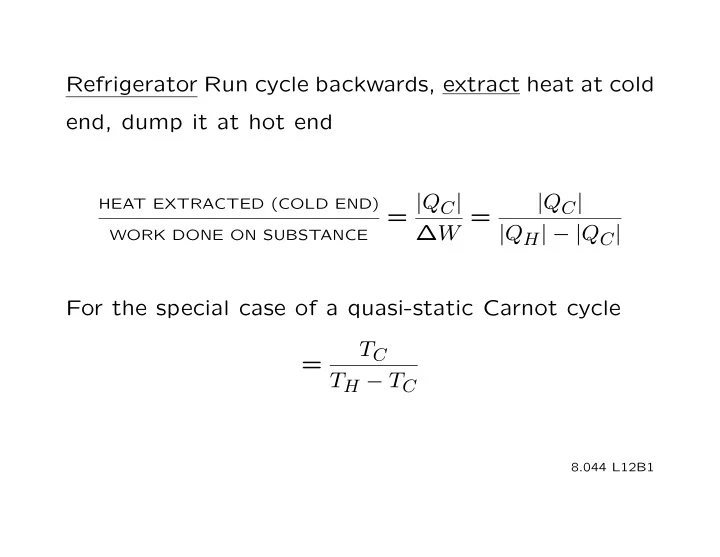
Refrigerator Run cycle backwards, extract heat at cold end, dump it at hot end

HEAT EXTRACTED (COLD END) WORK DONE ON SUBSTANCE

= |QC| ∆W = |QC| |QH| − |QC| For the special case of a quasi-static Carnot cycle TC = TH − TC

8.044 L12B1

• As with engine, can show Carnot cycle is optimum.
• Practical: increasingly difficult to approach T = 0.
• Philosophical:

T = 0 is point at which no more heat can be extracted.

8.044 L12B2

Heat Pump Run cycle backwards, but use the heat dumped at hot end.

HEAT DUMPED (HOT END) WORK DONE ON SUBSTANCE = |QH|

∆W = |QH| |QH| − |QC| For the special case of a quasi-static Carnot cycle TH = TH − TC

8.044 L12B3

55o 70o F subsurface temp. at 40o latitude TC = 286K F room temperature TH = 294K |QH| ∆W ≤ ∼ 37 294 8

8.044 L12B4

3rd law lim S = S0

T0

At T = 0 the entropy of a substance approaches a constant value, independent of the other thermody- namic variables.

• Originally a hypothesis
• Now seen as a result of quantum mechanics

Ground state degeneracy g (usually 1) ⇒ S → k ln g (usually 0)

8.044 L12B5

∂S Consequences = 0 ∂x

T=0

Example: A hydrostatic system 1

∂V

1

∂S

α ≡ = − as T 0 V ∂T

P

V ∂P

T

V Tα2 CP − CV = KT as T 0 S(T)−S(0) =

T

T=0

CV (T →) T → dT → CV (T) 0 as T 0

8.044 L12B6

Ensembles

• Microcanonical: E and N fixed

Starting point for all of statistical mechanics Difficult to obtain results for specific systems

• Canonical: N fixed, T specified; E varies

Workhorse of statistical mechanics

• Grand Canonical: T and µ specified; E and N vary

Used when the the particle number is not fixed

8.044 L12B7

If the density in phase space depends only on the energy at that point, ρ({p, q}) = ρ(H{p, q}), carrying out the indicated derivatives shows that ∂ρ = 0. ∂t This proves that ρ = ρ(H{p, q}) is a sufficient condition for an equilibrium probability density in phase space.

8.044 L7B2



√

 √

−1/2 −E/2<E>

 

p(px) = √ 3 e N e1/2 √ 1 e 4πm 3N < E > 1

−E/2<E>

= √ e 4πm < E > Now use E = p2/2m and < E >=< p2 > /2m.

x x

1

2 2

−p /2<p >

x

p(px) = e

x

2π < p2 >

x

8.044 L7B17

15

• d) Let Ω' be the volume in a phase space for N − 1 oscillators of total energy E − t where

t = (1/2m)pi

2 + (mω2/2)qi 2 . Since the oscillators are all similar, < t >= E/N = kT .

p(pi, qi) = Ω'/Ω Ω' 2π N−1 1 (E − t)N−1 = ω (N − 1)! −1 N Ω' 2π N! E − t 1 = Ω ω (N − 1)! E E − t

• N

ω N t = 1 − 2π E − t E ' v- " ' v- "

≈<E>−1 ≈exp[−E/<E>]

1 p(pi, qi) = exp[−t/ < t >] (2π/ω) < t >

2 2

= 1 exp[−pi /2mkT ] exp[−(mω2/2kT )qi ] (2π/ω)kT = √ 1 exp[−pi

2/2mkT ]

1 exp[−qi

2/2(kT/mω2)]

2πmkT 2π(kT/mω2) = p(pi) × p(qi) ⇒ pi and qi are S.I.

2 1 1 IS THE SUBSYSTEM OF INTEREST. 2, MUCH LARGER, IS THE REMAINDER OR THE "BATH". ENERGY CAN FLOW BETWEEN 1 AND 2. THE TOTAL, 1+2, IS ISOLATED AND REPRESENTED BY A MICROCANONICAL ENSEMBLE.

8.044 L12B8

For the entire system (microcanonical) one has

volume of accessible phase space consistent with X

p(system in state X) = Ω(E) In particular, for our case p({p1, q1}) ≡ p(subsystem at {p1, q1}; remainder undetermined) Ω1({p1, q1})Ω2(E − E1) = Ω(E)

8.044 L12B9

k ln p({p1, q1}) = k ln Ω1 + k ln Ω2(E − E1) − k ln Ω(E)

v v v

k ln 1 = 0 S2(E − E1) S(E) ∂S2(E2) S2(E − E1) ≈ S2(E) − E1 ∂E2

v

evaluated at E2 = E

8.044 L12B10

H1({p1, q1}) k ln p({p1, q1}) = − + S2(E) − S(E)

v

T

v

The first term on the right depends on the specific state of the subsystem. The remaining terms on the right depend on the reser- voir and the average properties of the subsystem.

8.044 L12B11

• In all cases, including those where the system is too

small for thermodynamics to apply, H1({p1, q1}) p({p1, q1}) exp[− ] kT H1({p1, q1}) exp[− ] kT = H1({p1, q1}) exp[− ]{dp1, dq1} kT

8.044 L12B12

If thermodynamics does apply, one can go further. S(E) = S1(< E1 >) + S2(< E2 >) S2(E) − S(E) = S2(E) − S2(< E2 >) −S1(< E1 >) , k j ≈ (∂S2(E2)/∂E2) < E1 >=< E1 > /T H1({p1, q1}) < E1 > k ln p({p1, q1}) = − + − S1 T T (< E1 > −TS1) H1({p1, q1}) p({p1, q1}) = exp[ ] exp[− ] kT kT , k j ≡ 1/Zhα

8.044 L12B13

• < E1 > −TS1 = U1 − T1S1 = F1

H({p, q}) p({p, q}) = (Zhα)−1 exp[− ] kT Z is called the partition function. H({p, q}) Z(T, V, N) = exp[− ]{dp, dq}/hα kT (E − TS) F (T, V, N) = exp[− ] = exp[− ] kT kT

8.044 L12B14

In the canonical ensemble, the partition function is the source of thermodynamic information. F(T, V, N) = −kT ln ZN(T, V ) ∂F S(T, V, N) = − ∂T V,N ∂F P(T, V, N) = − ∂V T,N

8.044 L12B15

MIT OpenCourseWare http://ocw.mit.edu

8.044 Statistical Physics I

Spring 2013 For information about citing these materials or our Terms of Use, visit: http://ocw.mit.edu/terms.